Flight
Test II
Excess Power and Rate of Climb Determination
For
The
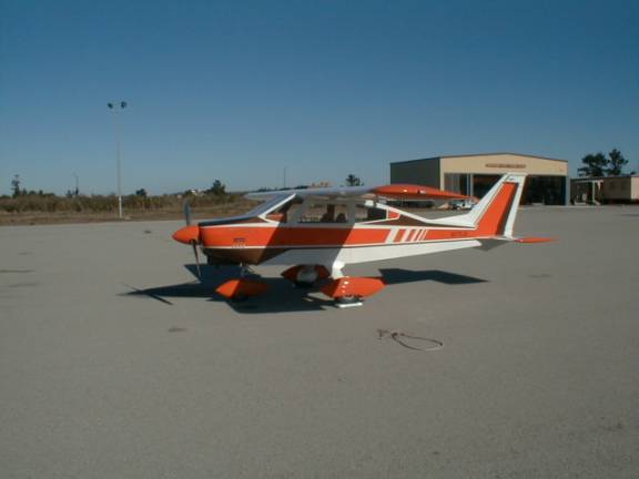
KOPP BD-4 N375JK “Miss Daisy”
By LT Kenneth G. Kopp
Co-Builder/Owner of the Kopp BD-4 “Miss Daisy”
Table of Contents
Part I - Instrument Position Errors
Level Acceleration Data (climb to altitude technique)
List of Figures
Figure 1 Airspeed Position Error Plot
Figure 2 Level Acceleration Techniques
Figure 3 Sawtooth Climb Method
Figure 6 R/C uncorrected test day 3000ft
Figure 8 Calculated Descent Rate Correction
Figure 9 R/C 3000ft 2200 lbs std day
Figure 10 Power Available vs. Power Required 3000ft
Figure 20 Climb Gradient Triangle
Figure 21 Gradient Temperature Dependence
Figure 23 Absolute and Service Ceilings
LIST OF TABLES
Table 1 Summary Table for Kopp BD-4
Table 2Kopp BD-4 Specifications
Table 3 Crew and altitude assignments
Table 4 Flight Responsibilities
Table 5 Level Acceleration 3000 feet
Table 6 DVpc & DHpc corrections
3000ft
Table 7 3000ft R/C reduced data
Table 8 Standard Day Climb Performance Values from plots
Table 10 Average Rate of Climb
Table 11 Averaged Aircraft Gross Weight
Table 12 Climb Angle and Gradient
Table 16 Absolute and Service Ceilings
Table 17 Performance Summary Table
Table 18 1500 ft level accel data
Table 21 Sawtooth reduced data
Introduction
This report represents the second in a series of planned flight tests for the purpose of determining performance and operating parameters of the Kopp manufactured BD-4 experimental (homebuilt) airplane. Flight Test 1 was conducted for determination of the drag polar and power required for level flight. Data was collected at various weights and altitudes and then standardized to sea level, max gross weight conditions during data reduction. This key information forms the foundation by which operational flight performance parameters are determined. A summary of the results obtained from Flight Test 1 are shown in the table below.
Table 1 Summary Table for Kopp BD-4
Altitude / Weight
|
Max Cl/Cd |
Min Thrust Required |
|
3000 ft / 1950 lbs |
8.8235 |
217.87 lbs |
|
7500 ft / 2130 lbs |
9.0329 |
229.63 lbs |
Parameters
|
Drag Polar
|
Power Curve
|
Cdo
|
0.0440
|
0.0425
|
e
|
0.7031
|
0.6507
|
|
Altitude |
Minimum
Thrust Horsepower Required |
|
|
3500
ft 1950 lbs |
52.33
HP |
|
|
7500
ft 2130 lbs |
60.59
HP |
|
|
Standardized
|
59.16
HP |
|
|
Kopp BD-4 Summary Table Test conducted 27 July, 2000 Data to be added upon further testing |
||
Performance parameters
calculated in table one are a result of airframe configuration only and are
independent of installed propulsion.
This flight test introduces propulsion system effects for determination
of relationships between the two independent data sets. At the conclusion of this report table 1 is
expanded to include: maximum rate-of-climb (R/Cmax), Vx
(max angle-of-climb airspeed), Vy (R/Cmax airspeed) and
max angle of climb (AOC).
Excess power, defined as the difference between power available and power required for level unaccelerated flight results in either a climb or an acceleration. Power available is determined by the installed propulsion system. Two data collection methods are employed for excess power determination, these are; level acceleration and sawtooth climb methods. Data collected is reduced to determine climb rate, excess power and in conjunction with power-required data, power available. The power available calculated from test data is compared to values determined using engine power charts and propeller performance mapping software supplied by Hartzell Propeller Inc. as a means to validate (or invalidate) the flight test method and the supplied propeller and engine data. Comparison between flight test methods is also included.
Three different altitudes,
1500ft, 3000ft and 7500ft were flown during the level acceleration test and a
single 3000ft flight was flown using the sawtooth climb method
The Kopp BD-4’s designed mission is that of medium range cross-country cruiser and general recreational aircraft. The main focus of these flight tests is to determine how its performance aids or deters fulfillment of its designed mission.
Kopp
BD-4
The Kopp BD-4 is a single
engine, 4 place IFR capable homebuilt airplane. It is equipped with a Lycoming
O-360-A1A 180 HP horizontally opposed, direct drive, normally aspirated engine
turning a 74” Hartzell 7666-2 constant speed propeller.
Wings
The BD-4 has a cantilever high wing with a 64-415 modified airfoil. A plain flap of 71% span and cord of 15% MAC can deflect from 0°-30°. Ailerons of the sealed configuration, also have a chord of 15% MAC and are deflected differentially by 1” diameter torque tubes. The unique tubular spar and metal-to-metal bonding used in the wings kept costs of construction and maintenance low, weight light and construction simple. Three components comprise the entire cantilever spar design; the center section and two slightly larger wing tubes which are all bolted together with four AN4 bolts ( not so jokingly referred to as Jesus bolts).
Fuselage
The all-metal fuselage was fabricated entirely of simple flat aluminum gussets and varying length angles of different dimension. The entire assembly is bolted together “erector set style” using the highest quality AN hardware. .020” 2024 T3 aluminum skin is bonded and blind riveted to the structure and together form a sturdy, dependable airframe rated to a limit load of +-6 g’s.
Empennage
The horizontal
tail is of the “all-flying” variety found on many Piper airplanes. The stabilator consists of a single tubular
spar and several rib sections formed into a 63-009 airfoil. The vertical tail is of similar
construction.
Table
2 below is a detailed listing of all
Kopp BD-4 specifications..
Table 2Kopp
BD-4 Specifications
Wing Span |
25.6 ft |
Cabin Width |
42” |
|
Wing Chord |
4 ft |
Cabin length |
89” |
|
Wing Area |
102.33 ft2 |
Cabin height |
41” |
|
Aspect Ratio |
6.4 |
Fuel Capacity |
60 gal |
|
Aileron Area |
3.5 ft2 |
Elevator Def up |
15° |
|
Flap Area |
8 ft2 |
Elevator Def down |
6° |
|
Flap Span |
71% |
Trim Tab Up |
18° |
|
Aileron Defl Up |
25° |
Trim Tab Down |
10° |
|
Aileron Defl Down |
17° |
Rudder Deflection |
+- 25° |
|
Length |
21.4 ft |
Flap Deflection |
0°-30° |
|
Horizontal Stab Span |
7.3 ft |
Max Gross Weight |
2200 |
|
Horizontal Chord |
3 ft |
Empty Weight |
1412 lbs |
|
Horizontal Stab Area |
21.9 ft2 |
Useful Load |
788 lbs |
|
Horizontal Stab AR |
2.4 |
Wing Loading |
21.5 lbs/ft2 |
|
Vertical Stab Area |
12 ft2 |
Power Loading |
12 lbs/BHP |
Part I
- Instrument Position Errors
Pitot static position errors were determined and reported
in flight test 1. Figure 1 below is a
plot of ΔVpc vs. Vias
(indicated) where ΔVpc represents the velocity correction
which when applied to Vias results in Vcas (calibrated
airspeed). Vcas is then
adjusted for test day density altitude to arrive at Vtas (true
airspeed).
Figure 1
Airspeed Position Error Plot
mph
These corrections are
important since the primary measurement sources during flight are the installed
aircraft pitot-static instruments (airspeed, altimeter) and without valid
corrections, results would be erroneous.
In addition to the airspeed correction the altimeter must also be
corrected according to the following relationship:
 , where ΔHpc is the correction applied to
indicated altitude as follows:
, where ΔHpc is the correction applied to
indicated altitude as follows:
Hi (indicated) +
ΔHpc= Hc (true altitude)
As can be seen by the
equation above, DHpc is dependent
upon altitude, requiring a correction to be applied to each recorded altitude throughout the airspeed range
flown, as indicated in the figure below.
Figure 2 Hpc Plot
Part II – Flight Test
General
Information
This test was conducted in the Kopp BD-4 on 10 Aug,
2000 departing from Monterey Peninsula Airport (MRY) at 10:00 am. Conditions at take-off were:
Wind: 290/8
Alt: 30.04
Sky Clear
Rwy: 28R
Crew and altitude assignments were as follows:
Table 3 Crew and altitude assignments
Crew - level acceleration runs
|
Altitude |
Gross Weight (approx) |
|
LT Ken Kopp / LT Anthony Fortesque |
3000 ft |
2175 lbs |
|
LT Ken Kopp / LT Anthony Fortesque |
7500 ft |
2130 lbs |
|
Crew – Sawtooth Climb |
Altitude |
Gross Weight (approx) |
|
LT Ken Kopp / Maj. Jim Hawkins |
3000 ft |
2025 lbs |
The test area was restricted to Salinas Valley from Salinas to 15 miles South East of King City. Crew coordination and a thorough test procedures briefing preceded each flight. Data collection sheets were developed, printed and discussed in detail prior to flight as well. Specific responsibilities were delegated as follows:
Table 4 Flight Responsibilities
|
Responsibility |
Pilot at the Controls |
Pilot Not at the Controls |
Flight Safety |
Primary |
Secondary |
|
Airwork |
Primary |
|
|
Test Procedure |
|
Primary |
|
Data Recording |
|
Primary |
|
Communications |
Primary |
Secondary |
|
Navigation |
Secondary |
Primary |
|
Visual Lookout |
Secondary |
Primary |
|
Emergencies |
Primary |
Secondary |
ATC flight following was utilized to the maximum extent possible to aid in collision
avoidance. King City and Salinas Muni were designated primary diverts in the event an emergency due to mechanical failure or weather occurred.
To minimize parallax error the left seat pilot remained at the controls while the right
seat pilot recorded data.
Level Acceleration Method
Climb to Altitude Technique
In this method the aircraft
is slowed to Vmca (minimum controllable airspeed) 2-3 hundred feet
below the target altitude. Full power
is smoothly applied and the aircraft allowed to climb. As the aircraft approaches target altitude a
pitch correction is applied to level the aircraft on target altitude while
accelerating to Vmax. Upon reaching altitude a timer is started and
elapsed time recorded at predetermined airspeed intervals. Pilot technique, solid crew coordination and
practice are required to obtain any degree of accuracy in this method. Indicated altitude should be maintained as
precisely as possible and any indicated rates of climb or descent should be
noted if possible. Data recorded is Hi, Vias, elapsed time, MP, RPM and OAT.
Constant
Altitude Technique
This
technique requires the aircraft to be slowed to Vmca at the
specified target altitude and to smoothly apply power while recording elapsed
time between specified airspeed intervals during the ensuing acceleration. This technique is extremely difficult in the
Kopp BD-4 due to torque effects on yaw and roll making altitude control
difficult during the first few seconds of data collection, therefore; the climb to altitude technique is
preferred.
Figure 2
Level Acceleration Techniques
Sawtooth Climb Method
In
this method a test band of ± 500 feet is set around a target altitude (3000ft
in this case) while the aircraft is slowed to Vmca 1-2 hundred feet
below the lower test band altitude. While maintaining constant Vias
, full power is applied and a climb commenced. Upon reaching the lower limit a
timer is started and elapsed time between
hundred foot intervals is recorded, along with Vias, MP, RPM
and OAT. This cycle is repeated at 5 mph airspeed intervals throughout the
range of interest.
Figure 3 Sawtooth Climb Method
Part III Data Reduction
Level Acceleration Data
(climb to altitude technique)
Measurements were recorded and reduced for indicated altitudes of 1500, 3000 and 7500 ft. Five runs were conducted for each altitude to facilitate averaging for the purpose of minimizing deviations during each run. A running fuel burn was tallied to account for change in gross weight over the test period. For purposes of brevity, only data for the 3000 feet case will be discussed in the body of the text, however; plots of all pertinent data will be displayed and discussed. The remaining data is located in the appendix.
Raw data collected during the 3000 ft run is displayed in the table below.
Table 5 Level Acceleration 3000 feet
|
Data Sheet |
|
3000 Ft |
|
|
|
|
|
Pwr Avail |
|
|
|
|
|
|
|
start fuel |
G W |
Wind |
Alt |
Temp |
Srt T |
T/O T |
|
60 |
2195 |
350/6 |
30.06 |
17 |
11:12 |
11:23 |
|
Climb pwr |
lvl T |
trans pwr |
Climb
BR |
Run
BR |
Transit
BR |
Descent BR |
|
27/27 |
11:27 |
27/20 |
13 |
13 |
7.8 |
5.0 |
|
|
|
|
|
|
|
|
|
PA |
OAT |
MP |
RPM |
Start GW |
End GW |
Ave GW |
|
3000 |
66 |
26.2” |
2700 |
2182.035 |
2165.0 |
2173.5 |
|
Clock TIme |
11:35 |
11:40 |
11:46 |
11:50 |
11:54 |
|
|
IAS |
Time |
Time |
Time |
Time |
Time |
Ave Time |
|
70 |
0 |
0 |
0 |
0 |
0 |
0.0 |
|
75 |
|
3 |
4 |
2 |
2 |
2.8 |
|
80 |
3 |
5 |
5 |
5 |
3 |
4.2 |
|
85 |
|
7 |
6 |
8 |
5 |
6.5 |
|
90 |
5 |
8 |
9 |
10 |
8 |
8.0 |
|
95 |
|
10 |
10 |
11 |
9 |
10.0 |
|
100 |
10 |
15 |
12 |
12 |
10 |
11.8 |
|
105 |
15 |
19 |
16 |
14 |
13 |
15.4 |
|
110 |
18 |
23 |
20 |
17 |
15 |
18.6 |
|
115 |
24 |
25 |
23 |
19 |
18 |
21.8 |
|
120 |
27 |
28 |
28 |
22 |
23 |
25.6 |
|
125 |
31 |
35 |
35 |
28 |
29 |
31.6 |
|
130 |
35 |
40 |
40 |
32 |
35 |
36.4 |
|
135 |
43 |
44 |
44 |
38 |
40 |
41.8 |
|
140 |
52 |
50 |
53 |
45 |
48 |
49.6 |
|
145 |
59 |
59 |
64 |
54 |
59 |
59.0 |
|
150 |
77 |
97 |
83 |
81 |
79 |
83.4 |
|
|
|
|
|
|
|
|
The first step in data reduction is to apply static position corrections to both airspeed and altitude as mentioned in part 1. The result of these corrections is displayed in the table below. Additionally, values for standard temperature, pressure and density for each true altitude (Hc) are computed via atmospheric table interpolation.
Table 6 DVpc & DHpc corrections 3000ft
|
3000ft |
rho std |
|
sigstd |
gama |
ao |
Ti |
|
|
|
|
|
0.0022 |
|
0.917722 |
1.4 |
1116.29 |
66 |
|
|
|
|
Vias |
Delt Vpc |
Vcas |
Hi |
delt Hpc |
Hc |
Ts |
Ps |
rho |
rho std |
|
mph |
mph |
mph |
ft |
ft |
ft |
F |
lb/ft^2 |
slug/ft^3 |
slug/ft^3 |
|
70 |
10.09 |
80.09 |
3000.00 |
51.54 |
3051.54 |
46.94 |
1893.29 |
0.002096268 |
0.002172 |
|
75 |
8.03 |
83.03 |
3000.00 |
43.93 |
3043.93 |
46.96 |
1893.83 |
0.002096858 |
0.002173 |
|
80 |
6.36 |
86.36 |
3000.00 |
37.13 |
3037.13 |
46.99 |
1894.30 |
0.002097385 |
0.002173 |
|
86 |
4.75 |
90.75 |
3000.00 |
29.82 |
3029.82 |
47.01 |
1894.81 |
0.002097952 |
0.002173 |
|
90 |
3.85 |
93.85 |
3000.00 |
25.31 |
3025.31 |
47.03 |
1895.13 |
0.002098301 |
0.002174 |
|
95 |
2.88 |
97.88 |
3000.00 |
19.96 |
3019.96 |
47.05 |
1895.50 |
0.002098716 |
0.002174 |
|
100 |
2.03 |
102.03 |
3000.00 |
14.79 |
3014.79 |
47.07 |
1895.86 |
0.002099116 |
0.002174 |
|
105 |
1.27 |
106.27 |
3000.00 |
9.72 |
3009.72 |
47.09 |
1896.22 |
0.002099509 |
0.002175 |
|
110 |
0.58 |
110.58 |
3000.00 |
4.69 |
3004.69 |
47.10 |
1896.57 |
0.002099899 |
0.002175 |
|
115 |
-0.03 |
114.97 |
3000.00 |
-0.29 |
2999.71 |
47.12 |
1896.92 |
0.002100285 |
0.002175 |
|
120 |
-0.59 |
119.41 |
3000.00 |
-5.17 |
2994.83 |
47.14 |
1897.26 |
0.002100663 |
0.002176 |
|
125 |
-1.08 |
123.92 |
3000.00 |
-9.86 |
2990.14 |
47.16 |
1897.59 |
0.002101026 |
0.002176 |
|
130 |
-1.50 |
128.50 |
3000.00 |
-14.24 |
2985.76 |
47.17 |
1897.90 |
0.002101366 |
0.002176 |
|
135 |
-1.84 |
133.16 |
3000.00 |
-18.18 |
2981.82 |
47.18 |
1898.17 |
0.002101671 |
0.002177 |
|
140 |
-2.10 |
137.90 |
3000.00 |
-21.55 |
2978.45 |
47.20 |
1898.41 |
0.002101933 |
0.002177 |
|
145 |
-2.29 |
142.71 |
3000.00 |
-24.28 |
2975.72 |
47.21 |
1898.60 |
0.002102144 |
0.002177 |
|
150 |
-2.40 |
147.60 |
3000.00 |
-26.34 |
2973.66 |
47.21 |
1898.74 |
0.002102304 |
0.002177 |
|
|
|
|
|
|
|
Interpolation
Values for 3000 ft |
|
|
|
|
|
|
|
|
|
|
A |
Ts |
Ps |
rho std |
|
|
|
|
|
|
|
2500 |
509.77 |
1931.9 |
0.0022079 |
|
|
|
|
|
|
|
3500 |
506.21 |
1861.9 |
0.0021429 |
Rate of climb, a measure of excess power, is calculated according to the equation below:
![]() , where Vtas is true airspeed in ft/sec and
dh/dt is the change in altitude with respect to time or R/C in ft/sec. dVtas/dt
is the acceleration.
, where Vtas is true airspeed in ft/sec and
dh/dt is the change in altitude with respect to time or R/C in ft/sec. dVtas/dt
is the acceleration.
With static position corrections applied
determination of Vtas for each data point is accomplished by
solving the equation below.
![]() , where σ is
the ratio of air density at each Hc to standard sea level
density. The slope of a tangent line
to the curve resulting from a plot of Vtas vs. time is equal to the
instantaneous acceleration at that point or dVtas/dt as shown in the figure below.
, where σ is
the ratio of air density at each Hc to standard sea level
density. The slope of a tangent line
to the curve resulting from a plot of Vtas vs. time is equal to the
instantaneous acceleration at that point or dVtas/dt as shown in the figure below.
To determine values of dVtas/dt
analytically, a third order curve fit is applied to the data plotted above. The
resulting equation is then differentiated with respect to time to generate an
equation for dVtas/dt as
shown below:
![]()
differentiating with respect
to time results in:
![]()
Applying the recorded times
during the flight to the above equation results in values of acceleration for
each data point as shown in the figure below.
Determination of uncorrected R/C for test day conditions and
gross weight requires only that the equation ![]() be solved for
each data point. The result of this calculation is displayed in the figure
below.
be solved for
each data point. The result of this calculation is displayed in the figure
below.
Figure 6
R/C uncorrected test day 3000ft
The R/C depicted above is termed
uncorrected because data leading to calculated values of acceleration is
corrupted by altitude management and static position errors during the run. A quick glance back at table 6 and figure 2 shows that although
indicated altitude Hi remained constant the aircraft is actually
descending as it accelerates.
In fact, 77.8 feet was lost during the run. A plot of Hc vs. Time for the run is shown in the figure below.
This actual R/D (rate of descent)
causes the aircraft to accelerate more quickly
resulting in an optimistically higher value of calculated dh/dt. Fortunately, this effect is easily corrected
by simply subtracting the actual R/D directly from calculated values of dh/dt to arrive at the airplanes actual R/C
climb under test day weight and atmospheric conditions. Several methods can be used to estimate the
R/D during the run. A curve fit of the
plot above can be differentiated to arrive at an equation for dh/dtlocal
. Unfortunately as the order of the fit increases so to does the sensitivity of
its derivative. For this reason, the
local R/D at each point was calculated by the following relationship:
![]() . Which is simply the
average slope between each two test points.
A plot of the determined descent rate is shown below.
. Which is simply the
average slope between each two test points.
A plot of the determined descent rate is shown below.
Figure 8
Calculated Descent Rate Correction
Test day R/C is then
determined by:
![]()
Test day R/C is useful for
validation of known data points or for comparison with similar test day
condition results, but to enable prediction of aircraft performance during
other than test day conditions , several standardizing corrections must be
applied to the calculated R/Ctest day. Otherwise, test data would be required for each weight, altitude
and temperature combination, which is unrealistic. The additional corrections are listed below in the order they are
to be applied.
- Power correction (DR/Cpower) – applied to account
for change in power generated due to non-standard temperature.
- Inertial correction (DR/Cinertial) – applied to account
for non-standard weight
- Induced drag correction (DR/Cind) – applied to account
for non-standard weight.
Knowing full power was used for all climb performance calculations, the power correction is determined by:
 , where Tstd can be any temperature of interest,
not necessarily standard atmospheric temperature.
, where Tstd can be any temperature of interest,
not necessarily standard atmospheric temperature.
and the inertial correction
by:
 , where Wstandard is any weight of interest.
Because an airplane flying
at higher gross weight must fly a
higher angle of attack for a given airspeed the induced drag of the heavier
plane will necessarily be higher. Recalling that induced drag is a function of
CL2 and CL is a function of lift, in level
unaccelerated flight lift equals the
weight of the aircraft. Therefore, as weight increases so does the value
of CL2 for a given airspeed and thus induced drag
increases as well. This results in more power required to maintain level flight
at the higher weight for that airspeed.
An increase in power required results in decreased excess power, since
installed power is independent of airframe aerodynamics and remains constant
for a given airspeed, resulting in a
decreased R/C. The induced drag
correction is given by:
 , where q is the dynamic pressure at the test altitude and
temperature. Combining test day R/C
with each correction for specified Wstd and Tstd results
in R/C corrected to those weights and temperatures and is given by:
, where q is the dynamic pressure at the test altitude and
temperature. Combining test day R/C
with each correction for specified Wstd and Tstd results
in R/C corrected to those weights and temperatures and is given by:
![]()
Arbitrarily choosing values of Wstd and Tstd
to be 2200 lbs and standard atmospheric temperature at each Hc
determined in table 6 and applying each correction to R/Ctest day, results in values of R/Cstd shown
in the following table.
Table 7 3000ft R/C reduced data
|
|
|
Ws (lbs) |
e |
AR |
S (ft^2) |
|
|
|
|
|
2200 |
0.7031 |
6.4 |
102.33 |
|
|
|
|
dh/dt |
climb/desc |
dh/dt |
Power |
inertial |
ind drag |
DH/DT |
|
Dv/dt |
uncorrected |
correction |
test day |
correction |
correction |
correction |
corrected |
|
(fps) |
(fpm) |
(fpm) |
(fpm) |
(fpm) |
(fpm) |
(fpm) |
(fpm) |
|
3.06 |
713.23 |
-166.01 |
547.22 |
27.55 |
-7.00 |
-16.28 |
551.49 |
|
2.97 |
715.94 |
-281.29 |
434.64 |
28.22 |
-5.64 |
-15.65 |
441.58 |
|
2.82 |
706.97 |
-190.83 |
516.14 |
28.81 |
-6.63 |
-15.06 |
523.26 |
|
2.72 |
709.73 |
-180.12 |
529.60 |
29.10 |
-6.80 |
-14.40 |
537.51 |
|
2.60 |
708.18 |
-160.56 |
547.62 |
29.91 |
-7.03 |
-13.80 |
556.70 |
|
2.49 |
707.43 |
-172.22 |
535.21 |
30.46 |
-6.89 |
-13.24 |
545.54 |
|
2.28 |
674.93 |
-84.57 |
590.35 |
31.01 |
-7.57 |
-12.71 |
601.09 |
|
2.10 |
647.85 |
-94.28 |
553.58 |
31.47 |
-7.12 |
-12.21 |
565.71 |
|
1.93 |
619.46 |
-93.35 |
526.11 |
31.76 |
-6.79 |
-11.75 |
539.33 |
|
1.74 |
580.08 |
-77.04 |
503.04 |
32.13 |
-6.52 |
-11.31 |
517.34 |
|
1.46 |
505.94 |
-46.89 |
459.05 |
32.50 |
-5.98 |
-10.90 |
474.67 |
|
1.26 |
452.41 |
-54.75 |
397.66 |
32.70 |
-5.24 |
-10.51 |
414.61 |
|
1.05 |
392.71 |
-43.77 |
348.93 |
32.90 |
-4.65 |
-10.14 |
367.04 |
|
0.80 |
308.64 |
-25.98 |
282.66 |
33.05 |
-3.84 |
-9.79 |
302.08 |
|
0.56 |
223.08 |
-17.41 |
205.67 |
33.26 |
-2.91 |
-9.46 |
226.56 |
|
0.26 |
109.45 |
-5.06 |
104.40 |
33.25 |
-1.68 |
-9.15 |
126.83 |
A plot of R/Ctest day and R/Cstd is shown in the figure on the next page.
Figure 9 R/C 3000ft 2200 lbs std day
Test Day: 2175 lbs, OAT 66° F
Normally, correcting the results
to Wstd equal to 2200 lbs would result in a decreased R/C, but test
day weight of 2175 lbs is only 25 lbs lighter than Wstd of 2200 lbs,
whereas, test day temperature was nearly 20° hotter resulting in a predicted increased R/Cstd.
The next step is to combine the calculated values of
excess power with power required data from the previous flight test. To do this, R/C must be converted to power
available according to the following relationship:
 , solving for PA (in HP)
 .
.
Combining the two plots
(power available and power required) requires the standardized power required
curve to be corrected to the same values of Wstd and Tstd
the R/C of data was corrected for previously,
otherwise results will not be valid.
An alternate method of calculating
power available is accomplished by multiplying the engine shaft
horsepower (SHP) by propeller
efficiency, η. The result of which is thrust horsepower available. The values of SHP are determined from
manifold and rpm settings cross-referenced to the manufactures power chart with
corrections for altitude and temperature applied. Propeller efficiencies were generated using Hartzell’s propeller
performance mapping software. A plot of
power available calculated using both methods and power required curve is shown on the next page.
Figure 10 Power Available vs. Power Required 3000ft
As can be seen from the plot
above, values of power available
calculated by multiplying shaft horsepower by prop efficiency intersects the
power required curve at Vmax as expected. Failure of the data calculated from rate of climb to intersect
this point is attributed to errors introduced in the data reduction process,
specifically when taking the derivative of curve fitted data, unaccounted for errors in instrumentation
and possibly weakness of the theory itself.
Reversing the above process to determine rate of climb (using the
SHP*η curve) to compare with the results measured during the test results
in the figure on the next page.
From
several hundred hours of experience in this particular aircraft the rate of
climb plot (yellow) derived from the engine and prop data is much more
representative of indicated climb rates
than those generated from level acceleration runs. Values of R/Cmax
(horizontal green line), Vy (vertical green line) and Vx (vertical
blue line) are determined graphically.
Maximum climb angle occurs when the ratio of R/C to horizontal velocity
is a maximum. Graphically this
corresponds to the intersection of a tangent line running through the origin as
depicted by the blue line. The maximum
climb angle is computed by:
 . , where Vx
is true airspeed in mph.
. , where Vx
is true airspeed in mph.
Similar plots for 1500 and 7500 feet are shown below:
Vy, Vx, R/Cmax, AOCmax
for all tested altitudes are shown in the table below.
Table 8 Standard Day Climb Performance Values from plots
|
Altitude
(ft) |
Vy
(mph) |
Vx
(mph) |
Max R/C (fpm) |
Max Climb Angle° |
|
1500 |
90 |
75 |
778 |
6.05 |
|
3000 |
90 |
75 |
740 |
5.907 |
|
7500 |
85 |
75 |
445 |
3.76 |
Sawtooth Climb
Similar methodology for data reduction is employed in this method. Static, power, inertial and induced drag corrections are applied as done previously. However, a few added corrections apply only to data measured in this manner. These corrections are:
- Tapeline (DR/Ctape) – due to non-standard
temp gradient
- Acceleration correction (DR/Caccel) – due to change in Vtas
during climb.
- Wind Gradient Correction (DR/Cwind) – due to wind effects.
Application of static position corrections is complicated in this case by the fact that altitude is changing continuously, therefore requiring the correction be applied at each recorded altitude and for each airspeed as shown in the table below:
|
gama= |
1.4 |
Ao= |
1116.3 |
|
True altitude for each
airspeed (Hc) |
|
||||
|
Indicated |
Vias |
70 |
75 |
80 |
85 |
90 |
95 |
100 |
110 |
120 |
|
altitude |
Vpc |
10.09 |
8.03 |
6.36 |
4.75 |
3.85 |
2.88 |
2.03 |
0.58 |
-0.59 |
|
2500 |
0.9316 |
2534.7 |
2529.6 |
2525.0 |
2519.9 |
2517.1 |
2513.5 |
2510.0 |
2503.2 |
2496.5 |
|
2600 |
0.928843882 |
2634.8 |
2629.7 |
2625.1 |
2619.9 |
2617.1 |
2613.5 |
2610.0 |
2603.2 |
2596.5 |
|
2700 |
0.926084388 |
2734.9 |
2729.8 |
2725.2 |
2720.0 |
2717.2 |
2713.6 |
2710.1 |
2703.2 |
2696.5 |
|
2800 |
0.923324895 |
2835.0 |
2829.9 |
2825.3 |
2820.1 |
2817.2 |
2813.6 |
2810.1 |
2803.2 |
2796.5 |
|
2900 |
0.920565401 |
2935.1 |
2930.0 |
2925.3 |
2920.1 |
2917.3 |
2913.7 |
2910.1 |
2903.2 |
2896.5 |
|
3000 |
0.917805907 |
3035.2 |
3030.1 |
3025.4 |
3020.2 |
3017.3 |
3013.7 |
3010.2 |
3003.2 |
2996.4 |
|
3100 |
0.915080169 |
3135.3 |
3130.1 |
3125.5 |
3120.2 |
3117.4 |
3113.7 |
3110.2 |
3103.2 |
3096.4 |
|
3200 |
0.91235443 |
3235.4 |
3230.2 |
3225.6 |
3220.3 |
3217.4 |
3213.8 |
3210.2 |
3203.2 |
3196.4 |
|
3300 |
0.909628692 |
3335.5 |
3330.3 |
3325.6 |
3320.4 |
3317.5 |
3313.8 |
3310.3 |
3303.2 |
3296.4 |
|
3400 |
0.906902954 |
3435.7 |
3430.4 |
3425.7 |
3420.4 |
3417.5 |
3413.9 |
3410.3 |
3403.2 |
3396.4 |
|
3500 |
0.904177215 |
3535.8 |
3530.5 |
3525.8 |
3520.5 |
3517.6 |
3513.9 |
3510.3 |
3503.3 |
3496.4 |
|
|
Sigma std |
|
|
|
|
|
|
|
|
|
The uncorrected average R/C for each airspeed is
then determined by dividing the difference between measured true altitudes by Dtime. 
The result of this calculation is shown in the table
below.
Table 10 Average Rate of Climb
|
|
|
Average |
Rate of |
Climb |
|
|
|
|
|
|
Altitude |
70 |
75 |
80 |
85 |
90 |
95 |
100 |
110 |
120 |
|
2600 |
731.57 |
762.09 |
923.76 |
612.61 |
1035.01 |
689.93 |
1200.36 |
833.41 |
|
|
2700 |
747.97 |
770.90 |
723.43 |
1035.10 |
882.80 |
645.42 |
789.71 |
625.06 |
299.97 |
|
2800 |
693.56 |
717.48 |
1035.26 |
577.27 |
968.24 |
472.63 |
521.90 |
882.44 |
681.75 |
|
2900 |
818.30 |
481.97 |
1154.72 |
698.09 |
682.17 |
689.94 |
480.15 |
833.41 |
454.50 |
|
3000 |
721.92 |
687.12 |
800.61 |
833.84 |
612.56 |
822.26 |
638.49 |
571.48 |
555.50 |
|
3100 |
650.03 |
813.74 |
779.81 |
750.45 |
800.41 |
909.46 |
857.40 |
705.95 |
571.37 |
|
3200 |
638.97 |
928.19 |
857.80 |
870.09 |
612.56 |
895.89 |
1091.24 |
759.57 |
799.91 |
|
3300 |
554.09 |
678.58 |
594.51 |
811.30 |
750.39 |
769.55 |
822.17 |
631.64 |
705.81 |
|
3400 |
681.00 |
792.28 |
706.43 |
645.56 |
582.83 |
845.42 |
659.54 |
600.06 |
491.75 |
|
3500 |
691.19 |
753.51 |
594.52 |
741.20 |
682.18 |
857.50 |
895.80 |
526.37 |
472.39 |
|
|
692.86 |
738.59 |
817.09 |
757.55 |
760.92 |
759.80 |
795.68 |
696.94 |
559.22 |
The bold faced values along the bottom row of the
chart are the averaged rate of climbs for each airspeed from 70-120 mph. At this point the values are corrected only
for static position errors.
Because altimeters, the
primary data source in this method, are calibrated to changes in static
pressure at standard sea-level conditions, circumstances in which temperature
is non-standard introduces errors in Hi. To correct for these errors the following equation is applied:
The next correction to be applied is the power correction used to compensate for variations in engine output with changes in inlet temperatures. This correction is applied in the same manner as was done during level acceleration runs.
During the climb static ambient pressure decreases as does temperature (normally), therefore air density decreases as altitude increases according to the equation of state:

as ρ decreases the value of σ, σ =
(ρ/ρsea level), decreases and since ![]() , Vtas increases with altitude. Therefore while
climbing at constant Vias (or Vcas) , Vtas is
increasing with altitude, hence the term flight path acceleration error. The
correction for this error is determined by:
, Vtas increases with altitude. Therefore while
climbing at constant Vias (or Vcas) , Vtas is
increasing with altitude, hence the term flight path acceleration error. The
correction for this error is determined by:
 .
.
The wind gradient was
neglected in this test because an accurate method for wind speed determination
was not available on test day. An
effective and simple method for determining the wind gradient, change in wind
speed with altitude, is through use of GPS ground speed calculation. Subtracting Vground from Vtas
results in wind velocity. The slope of a plot of wind velocity for each
altitude determines the wind gradient.
The wind gradient correction is given by:
![]()
Because the weight of the
aircraft is continuously decreasing during the test a weight correction must be
applied to maintain validity of the results.
Consulting manufactures fuel consumption charts to retrieve consumption
rates during the test and using real times recorded during each run allowed the
following table of tabulated gross weights to be generated.
Table 11 Averaged Aircraft Gross Weight
|
Aircraft
Weight Data |
Ws= |
2200 |
AR= |
6.4 |
e= |
0.7031 |
s= |
102.33 |
|
|
Climb burn Rate |
13 |
|
|
|
|
|
0.6507 |
|
|
|
Descent BR |
5 |
|
|
|
|
|
|
|
|
|
IAS (mph) |
70 |
75 |
80 |
85 |
90 |
95 |
100 |
110 |
120 |
|
start GW |
2028.91 |
2025.32 |
2021.80 |
2018.37 |
2014.87 |
2011.94 |
2009.00 |
2006.06 |
2002.46 |
|
End GW |
2026.76 |
2023.27 |
2019.91 |
2016.37 |
2012.86 |
2009.92 |
2006.99 |
2003.89 |
1999.90 |
|
Ave GW |
2027.84 |
2024.30 |
2020.85 |
2017.37 |
2013.87 |
2010.93 |
2008.00 |
2004.98 |
2001.18 |
Finally, corrections for
non-standard weight (inertial and induced drag) applied to the level
acceleration data is also applied here to result in standard day rate of climb
corrected for static, power, flight path acceleration, weight, inertial and
induced drag effects. A plot of
sawtooth generated R/C is shown in the figure below. The complete data table and results can be found in the appendix.
Notice both Vy and Vx agree
well with level acceleration data.
However, data points are not very smooth by any means. This could be attributed to the neglected
wind gradient correction, errors in temperature measurement and quite possibly
the airplane itself may exhibit nonlineararities at various points within its
envelope (no pilot error noted during data collection!). To check the validity of one method over the
other, a combined plot of standard day and weight R/C for both level
acceleration and sawtooth climb techniques is shown in the figure on the next
page.
This plot shows
nice agreement between the sawtooth and the R/C curve calculated from
SHP*η at 3000 feet. The 3000ft
level acceleration run however does not match well with the other data, thereby
confirming the common understanding this method is not desirable for low
performance aircraft.
Having now
validated the method of using engine charts and prop software to determine
power available, the next step is to find usefulness for the information
generated.
Data Application
With the data thus presented
the task at hand is to put it into useful form for operational use. Excess power has important effects on
aircraft performance and is a particularly important aspect of the preflight
planning phase of any flight. Pilots
must determine whether or not the aircrafts performance will ensure safe
operation in the environment in which they will be operating. Cross-country flying requires detailed
planning to increase the likelihood of a successful trip. All to often complacent pilots set out on a
journey not having consulted current conditions and aircraft performance
specifications as to whether the aircraft can indeed meet the performance
required to ensure a safe outcome. Climb
gradient, time to climb and fuel to climb are all very
important considerations which must be reviewed prior to flying in unfamiliar
territory or under adverse weather conditions. The purpose of this section is
to transform test data to useful information for safer and more consistent
operation.
Before
the information can be transformed however, it is first necessary to develop
relationships between the data collected over a broader range of altitudes and
weights. By tabulating and plotting the values of R/Cmax for each
altitude tested (1500, 3000, 7500ft) while varying the Wstd corrections over a range of gross weights
from 1800-2200, the relationship between R/Cmax and altitude is
generated for fixed gross weight. Next a plot of R/Cmax vs. weight
is generated for each of the three tested altitudes to generated a relationship
between R/Cmax and weight
for a fixed altitude. Curve fit
equations are generated and applied to a range of weights and altitudes thus
generating a table of R/Cmax for the weights and altitudes of
concern. These relationships are then
applied to R/Caocmax to determine the climb angles at various
weights and altitude as well.
These plots are shown in the figures below.
Climb Gradient
Climb gradient is a very important performance parameter to consider especially when conducting Standard Instrument Departure (SIDs) procedures under instrument meteorological conditions (IMC). Often SIDs specify the aircraft be able to maintain a minimum climb gradient until a specific point is reached on the departure to ensure adequate obstacle clearance with ground or man-made objects. For example, a note written in the SECA2 departure from Monterey Peninsula Airport (KMRY) states,
“Note: This SID requires a minimum climb of 405’ per
NM to 4000’”. This is due to close
proximity of the departure course to Jacks Peak, a 3300 ft mountain. Solving
for maximum climb gradient requires the maximum climb angle to be known for
each altitude and weight of interest.
Maximum climb angle is determined as previously discussed. Once obtained, climb gradient is determined
by solving the trigonometry problem depicted below:
Figure 20
Climb Gradient Triangle
R/Caocmax Horizontal Distance Traveled (nm)


![]()
The tables below show the result of this calculation.
Table 12 Climb Angle and Gradient
|
Max Climb Angle (deg)
std day |
|
|
|
|
Altitude |
|
|
|
|
|
|||
|
Weight |
0 |
1000 |
2000 |
3000 |
4000 |
5000 |
6000 |
7000 |
8000 |
9000 |
10000 |
11000 |
12000 |
|
1800 |
8.51 |
8.22 |
8.10 |
7.86 |
7.50 |
7.02 |
6.42 |
5.70 |
4.86 |
3.90 |
2.82 |
1.62 |
0.30 |
|
1900 |
7.81 |
7.52 |
7.40 |
7.16 |
6.80 |
6.32 |
5.72 |
5.00 |
4.16 |
3.20 |
2.12 |
0.92 |
-0.40 |
|
2000 |
7.11 |
6.82 |
6.70 |
6.46 |
6.10 |
5.62 |
5.02 |
4.30 |
3.46 |
2.50 |
1.42 |
0.22 |
-1.10 |
|
2100 |
6.41 |
6.12 |
6.00 |
5.76 |
5.40 |
4.92 |
4.32 |
3.60 |
2.76 |
1.80 |
0.72 |
-0.48 |
-1.80 |
|
2200 |
5.71 |
5.42 |
5.30 |
5.06 |
4.70 |
4.22 |
3.62 |
2.90 |
2.06 |
1.10 |
0.02 |
-1.18 |
-2.50 |
|
|
|
|
|
|
|
|
|
|
|
|
|
|
|
|
Max Climb Gradient
ft/nm std day |
|
|
|
Altitude |
|
|
|
|
|
||||
|
Weight |
0 |
1000 |
2000 |
3000 |
4000 |
5000 |
6000 |
7000 |
8000 |
9000 |
10000 |
11000 |
12000 |
|
1800 |
909 |
878 |
865 |
839 |
800 |
748 |
684 |
607 |
517 |
415 |
300 |
172 |
32 |
|
1900 |
833 |
802 |
789 |
763 |
725 |
673 |
609 |
532 |
442 |
340 |
225 |
98 |
-42 |
|
2000 |
758 |
727 |
714 |
688 |
650 |
598 |
534 |
457 |
368 |
266 |
151 |
24 |
-116 |
|
2100 |
683 |
652 |
639 |
613 |
575 |
523 |
459 |
383 |
293 |
191 |
77 |
-50 |
-190 |
|
2200 |
608 |
577 |
564 |
538 |
500 |
449 |
385 |
308 |
219 |
117 |
3 |
-125 |
-265 |
|
Add/subtract
4 ft/nm for every 30 degrees above/below standard atmospheric temperature. |
|
||||||||||||
Gradient temperature dependence curve is shown in the figure below.
Figure 21 Gradient Temperature Dependence
Time to Climb
Time
to climb information is useful for choosing optimum cruising altitudes for
given wind conditions in consideration of the total distance to be
traveled. Assuming the climb will be
conducted @ Vy and under maximum power, the time to climb can be
determined by:
graphically this is determined by calculating the
area under the curve of 1/(R/Cmax) vs. altitude as shown below:
Time to Climb
Integrating the six order polyfit
curve and applying the altitude and weight relationships determined previously
results in the following R/Cmax and Time to Climb tables.
|
|
|
|
|
|
|
Max R/C |
|
|
|
|
|
|
|
|
|
|
|
|
|
|
Altitude (ft) |
|
|
|
|
|
|
|
|
weight (lb) |
0 |
1000 |
2000 |
3000 |
4000 |
5000 |
6000 |
7000 |
8000 |
9000 |
10000 |
11000 |
12000 |
|
1800 |
1150 |
1143 |
1123 |
1092 |
1048 |
993 |
925 |
846 |
754 |
651 |
535 |
408 |
268 |
|
1900 |
1063 |
1055 |
1036 |
1004 |
961 |
905 |
838 |
758 |
667 |
563 |
448 |
320 |
181 |
|
2000 |
975 |
967 |
948 |
916 |
873 |
817 |
750 |
670 |
579 |
475 |
360 |
232 |
93 |
|
2100 |
887 |
880 |
860 |
829 |
785 |
730 |
662 |
583 |
491 |
388 |
272 |
145 |
5 |
|
2200 |
799 |
792 |
772 |
741 |
697 |
642 |
574 |
495 |
403 |
300 |
184 |
57 |
|
|
|
|
|
|
|
Time to Climb @ Vy full
power |
minutes |
|
|
|||||
|
|
0 |
1000 |
2000 |
3000 |
4000 |
5000 |
6000 |
7000 |
8000 |
9000 |
10000 |
11000 |
12000 |
|
1800 |
0 |
0.9 |
1.8 |
2.7 |
3.6 |
4.6 |
5.6 |
6.7 |
8.0 |
9.4 |
11.1 |
13.2 |
16.2 |
|
1900 |
0 |
0.9 |
1.9 |
2.9 |
3.9 |
5.0 |
6.1 |
7.4 |
8.8 |
10.4 |
12.4 |
15.0 |
19.0 |
|
2000 |
0 |
1.0 |
2.1 |
3.1 |
4.3 |
5.4 |
6.7 |
8.1 |
9.7 |
11.6 |
14.0 |
17.4 |
23.6 |
|
2100 |
0 |
1.1 |
2.3 |
3.5 |
4.7 |
6.0 |
7.5 |
9.1 |
10.9 |
13.2 |
16.2 |
21.0 |
34.4 |
|
2200 |
0 |
1.3 |
2.5 |
3.9 |
5.2 |
6.7 |
8.4 |
10.3 |
12.5 |
15.3 |
19.5 |
27.8 |
|
Assuming a full power climb @ Vy and
consultation of fuel consumption charts allows calculation of the amount of
fuel burned during the climb as shown in the table below.
|
|
|
|
|
Fuel to climb @ Vy max power |
13 gal /hr |
|
|
||||||
|
GW |
0 |
1000 |
2000 |
3000 |
4000 |
5000 |
6000 |
7000 |
8000 |
9000 |
10000 |
11000 |
12000 |
|
1800 |
0 |
0.2 |
0.4 |
0.6 |
0.8 |
1.0 |
1.2 |
1.5 |
1.7 |
2.0 |
2.4 |
2.9 |
3.5 |
|
1900 |
0 |
0.2 |
0.4 |
0.6 |
0.8 |
1.1 |
1.3 |
1.6 |
1.9 |
2.3 |
2.7 |
3.2 |
4.1 |
|
2000 |
0 |
0.2 |
0.4 |
0.7 |
0.9 |
1.2 |
1.5 |
1.8 |
2.1 |
2.5 |
3.0 |
3.8 |
5.1 |
|
2100 |
0 |
0.2 |
0.5 |
0.8 |
1.0 |
1.3 |
1.6 |
2.0 |
2.4 |
2.9 |
3.5 |
4.6 |
7.5 |
|
2200 |
0 |
0.3 |
0.5 |
0.8 |
1.1 |
1.5 |
1.8 |
2.2 |
2.7 |
3.3 |
4.2 |
6.0 |
|
Absolute and Service
Ceilings
Determination
of absolute and service ceilings is a simple matter of plotting altitude vs.
R/Cmax and noting the intersection of the resulting curve on the
altitude scale as shown in the figure below.
Figure 23
Absolute and Service Ceilings
Service
Ceiling (100 fpm)![]()
![]()
![]()
![]()
![]()
![]()
![]()
Table 16 Absolute and Service Ceilings
|
Weight |
1800 |
1900 |
2000 |
2100 |
2200 |
|
Service Ceiling (ft) |
13,200 |
12,600 |
12,000 |
11,400 |
10,600 |
|
Absolute Ceiling (ft) |
14,000 |
13,500 |
12,600 |
12,000 |
11,400 |
These
values match very well with actual altitude limits experienced during several
hundred flying hours in this airplane.
Conclusions
With
the data and tables calculated in this report operation of the Kopp BD-4 can be
conducted in a more safe and consistent manner. Level acceleration runs are both challenging to fly and limited
in their ability to offer accurate data for relatively low performance aircraft
such as this (it kills me to say this).
Further sawtooth climb testing would enable further validation of the
engine power charts and propeller mapping software. Data can now be added to the summary table as shown below.
Table 17 Performance Summary Table
Altitude / Weight
|
Max Cl/Cd |
Min Thrust Required |
|
3000 ft / 1950 lbs |
8.8235 |
217.87 lbs |
|
7500 ft / 2130 lbs |
9.0329 |
229.63 lbs |
Parameters
|
Drag Polar
|
Power Curve
|
Cdo
|
0.0440
|
0.0425
|
e
|
0.7031
|
0.6507
|
|
Altitude |
Minimum
Thrust Horsepower Required |
|
|
3500
ft 1950 lbs |
52.33
HP |
|
|
7500
ft 2130 lbs |
60.59
HP |
|
|
Standardized
|
59.16
HP |
|
|
Vx
(ias) |
75
mph |
|
|
Vy
(ias) |
90
mph |
|
|
R/Cmax
S.L max GW |
799
fpm |
|
|
AOCmax
S.L. max GW |
5.71° |
|
|
Service
Ceiling @ max GW |
10,600
ft |
|
|
Absolute
Ceiling @ max GW |
11,400
ft |
|
|
Kopp BD-4 Summary Table Test conducted 27 July, 2000 Data to be added upon further testing |
||
Flight test three will be conducted for the purpose
of neutral point determination for longitudinal static stability determination.