Flight Test I

Drag Polar / Power Required

For

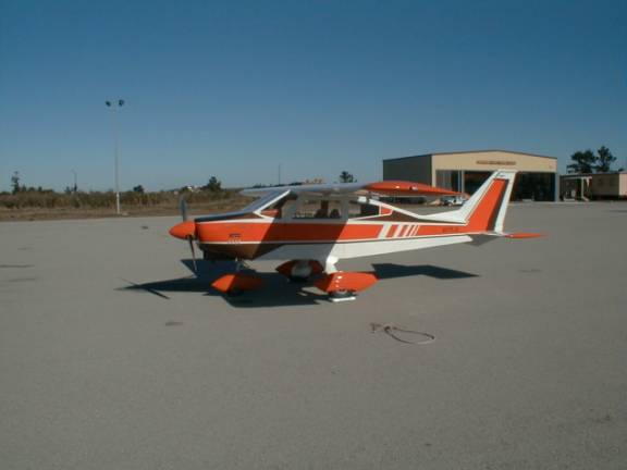
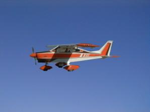
The KOPP BD-4 N375JK “Miss Daisy”

By LT Kenneth G. Kopp

CO-Builder/Owner of the Kopp BD-4 “Miss Daisy”

Table of Contents

List of figures. 3

Introduction.. 4

Kopp BD-4. 5

Wings. 5

Fuselage. 5

Empennage. 6

Mission.. 6

Part I - Instrument Position Errors.. 7

DV_pc Determination.. 9

DV_pc Flight Test.. 11

Part II – Drag Polar / Power Required.. 17

Flight Test Procedure. 18

Drag Polar / Power Required Flight Test.. 19

Flight Safety. 19

Data Analysis.. 27

Drag Polar.. 27

Power-required.. 34

Summary and Conclusions. 44

Appendix A.. 46

Appendix B.. 47

List of figures

Figure 1 Airspeed Position Error Plot.. 12

Figure 2 Vcas vs. Vias (mph) 13

Figure 3 Ps. 14

Figure 4 Hpc Plot.. 15

Figure 5 Propeller Thrust vs. Airframe Thrust Required.. 26

Figure 6 Drag Polar.. 28

Figure 7 Cd vs. Cl^2. 30

Figure 8 Calculated Drag Polar.. 31

Figure 9 Cl / Cd.. 33

Figure 10 THP vs Vtas (mph) 35

Figure 11 Normalized Power Required.. 37

Figure 12 Normalized Power Required (curve fit) 38

Figure 13 Power Curve. 40

Figure 14 Normalized Drag Polar.. 41

Figure 15 Prop efficiency.. 47

LIST OF TABLES

Table 1Kopp BD-4 Specifications. 6

Table 2 Calibrated Airspeed Data.. 11

Table 3 Crew and altitude assignments. 19

Table 4 Flight Responsibilities. 19

Table 5. 3000 ft Data.. 20

Table 6 Data Reduction for 3000 feet PA.. 22

Table 7 Error Corrections for 3000 ft.. 24

Table 8 Cdo and e. 30

Table 9. Max Lift / Drag.. 32

Table 10 Minimum Power-required.. 35

Table 11Cdo and e comparisons. 40

Table 12 Performance Table. 42

Table 13 Summary.. 44

Table 14 7500 ft Data and Reduction.. 46

Table 15 Instrument Corrections for 7500 ft.. 47

Introduction

The purpose of this report is to formally release findings and conclusions conducted during initial flight test of the experimental homebuilt Kopp BD-4 depicted on the title page. This is the first of an extensive series of planned flight tests and reports to be generated while investigating the flight characteristics and handling qualities of this airplane. Specific objectives include:

• Determine measurement accuracies (DV_pc & DH_pc)
• Determine the Drag Polar (C_L vs. C_D)
• Develop Power Required Curves
• Estimate (L/D)_max
• Determine minimum power required, maximum range and endurance airspeeds.

The test was conducted in two parts. Part one consisted of instrument position error determination using the course-over-ground method. Part two consisted of drag polar and power required data collection conducted at different altitudes and gross weights. Results of each test were tabulated and reduced using Microsoft Excel and MATLAB 5.03. Plots of all pertinent data along with the data itself is included within this report.

Kopp BD-4

The Kopp BD-4 is a single engine, 4 place, and IFR capable homebuilt airplane. It is equipped with a Lycoming O-360-A1A 180 HP horizontally opposed, direct drive, normally aspirated engine turning a 74” Hartzell 7666-2 constant speed propeller.

Wings

The BD-4 has a cantilever high wing with a 64-415 modified airfoil. A plain flap of 71% span and cord of 15% MAC can deflect from 0°-30°. Ailerons of the sealed configuration, also have a chord of 15% MAC and are deflected differentially by 1” diameter torque tubes. The unique tubular spar and metal-to-metal bonding used in the wings kept costs of construction and maintenance low, weight light and construction easy. Three components comprise the entire cantilever spar design; the center section and two slightly larger wing tubes which are all bolted together with four AN4 bolts ( not so jokingly referred to as Jesus bolts).

Fuselage

The all-metal fuselage was fabricated entirely of simple flat aluminum gussets and varying length angles of different dimension. The entire assembly is bolted together “erector set style” using the highest quality AN hardware. .020” 2024 T3 aluminum skin is bonded and blind riveted to the structure and together form a sturdy, dependable airframe rated to a limit load of +-6 g’s.

Empennage

The horizontal tail is of the “all-flying” variety found on many Piper airplanes. The stabilator consists of a single tubular spar and several rib sections formed into a 63-009 airfoil. The vertical tail is of similar construction.

Table 1 below is a detailed listing of all Kopp BD-4 specifications..

Table 1Kopp BD-4 Specifications

Wing Span	25.6 ft	Cabin Width	42”
Wing Chord	4 ft	Cabin length	89”
Wing Area	102.33 ft^2	Cabin height	41”
Aspect Ratio	6.4	Fuel Capacity	60 gal
Aileron Area	3.5 ft^2	Elevator Def up	15°
Flap Area	8 ft^2	Elevator Def down	6°
Flap Span	71%	Trim Tab Up	18°
Aileron Defl Up	25°	Trim Tab Down	10°
Aileron Defl Down	17°	Rudder Deflection	+- 25°
Length	21.4 ft	Flap Deflection	0°-30°
Horizontal Stab Span	7.3 ft	Max Gross Weight	2200
Horizontal Chord	3 ft	Empty Weight	1412 lbs
Horizontal Stab Area	21.9 ft^2	Useful Load	788 lbs
Horizontal Stab AR	2.4	Wing Loading	21.5 lbs/ft^2
Vertical Stab Area	12 ft^2	Power Loading	12 lbs/BHP

Mission

The Kopp BD-4’s designed mission is that of medium range cross-country cruiser and general recreational aircraft. The main focus of these flight tests will be to determine how its performance aids or deters fulfillment of its designed mission.

Part I - Instrument Position Errors

Prior to any serious flight test it is necessary to determine accuracies of all measurements taken during data collection. Determination of and documenting these accuracy leads to a more quantitative analysis of the airplanes performance and helps ensure more consistent and meaningful results. Because the performance of the Kopp BD-4 falls well below the accepted speed threshold of M=.3, where effects of compressibility become significant, all calculations will assume incompressible flow. The instrumentation used for this test consists of the installed primary flight performance instruments, which include airspeed (a/s), altimeter (alt), vertical speed indicator (vsi) and the outside air temperature gauge (oat). With the exception of OAT the most common source of error for the remaining instruments are those related to the static pressure port position, hence the term static position error is used. Because the A/S, Alt and VSI indicators all operate by measuring static ambient pressure via the static port, differences between actual ambient pressure and the pressure sensed by the instrument results in an error indicated by the individual instrument. Unfortunately it is very difficult, if not impossible, to position the static port such that no errors in measurement of static ambient pressures, P_s, are introduced during all flight regimes. Because the static port is usually located along the fuselage, sensed static pressure, P^{`</sup><sub>s,</sub> will vary as fuselage boundary layer conditions vary. Therefore; errors introduced because of static port position also vary with flow conditions. For this reason the difference between P<sub>s</sub> and P<sup>`}_s or DP_s, must be calculated throughout the airplanes complete range of airspeeds and configurations (flaps up and down, gear up and down, etc…). Additionally each instrument has an internal error called instrument error that must be determined by the manufacturer or tested in a calibrated laboratory environment. To achieve the highest degree of accuracy when reducing the data collected a correction factor for each error source must be applied to the recorded (indicated) data. DP_s is difficult to measure directly without additional costly equipment. Instead it is much simpler to determine the position error of a single indicator, such as A/S, and mathematically relate this to the others to determine their errors as well. Once individual indicator position errors are determined, DP_s can be solved analytically. The two primary indicator correction factors are DV_pc and DH_pc for the A/S and Altimeters respectively. Once these factors are obtained the following sequence is used to correct the data:

V_i Indicated airspeed (as read on the gauge)

+DV_ic instrument correction (from lab)

=V_ic Indicated corrected airspeed

+DV_pc static position correction

= V_cal Calibrated Airspeed

+ DV_comp compressibility correction (for M>.3)

= V_e Equivalent airspeed

/ correction for density at flight condition with reference to standard sea level density

= V_¥ True Airspeed, actual flight speed[1]

For altitude corrections:

H_i indicated pressure altitude (set to 29.92)

+DH_ic instrument correction (from lab)

= H_ic Indicated Pressure Altitude corrected for inst. error.

+DH_pc Position Error correction for static position error.

= H_c Calibrated Pressure Altitude.

DV_pc Determination

The ground-course method was chosen to determine DV_pc for the Kopp BD-4 due to its simplicity and because it requires no additional support equipment unlike other commonly used methods such as the tower-fly-by and trailing-bomb techniques. The ground-course flight procedure and data reduction is outlined below:

• Pick two easily identifiable (from the air) points 4-6 sm apart. Preferably along a stretch of straight road or highway as represented below:

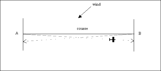
• Fly constant course between points A & B at 5 mph intervals from V_s1+5 to V_max.
• Record H_i (29.92), V_i, T_i and the time between points in both directions for each V_i.
• Maintain altitude and heading during each run. Allow airplane to drift with cross wind.
• Determine V_ground for each run by dividing the known distance between points A & B by the elapsed time to transit the two points. The result is the actual speed over the ground flown during the leg.
• Determine true velocity, V_tas, from 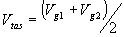. V_tas = V_ground in still air, therefore averaging groundspeeds has the effect of eliminating (or minimizing) the effect of wind when timing the runs, thereby providing a means for determination of actual true airspeed. To fully minimize effects of wind, it is advisable to fly in the early morning or late evening when winds are generally much calmer.[2] Also, a direct crosswind is better than a pure head or tailwind.
• Using the equation of state , determine the air density at H_p. Pressure, P is determined from H_p using standard atmosphere tables, T_i is the outside ambient air temperature read on the OAT gauge. At low mach numbers correction of T_i for stagnation effects results in minimal accuracy gain.
• Solve for V_e by using the formula
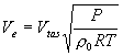
• Because M<.3 it is assumed V_e = V_c.
• DV_pc= V_c - V_i

DV_pc Flight Test

Flight test to determine DV_pc was conducted 11 November, 1999 over a 4.17 statute mile section of hwy 101 between Salinas and Soledad, California. During preflight chart study two bridges located at prominent intersections along the course to be flown were chosen as start and stop points for each run. Each run was conducted in the clean configuration (flaps up). A Magellan 3000XL handheld GPS was used to refine the charted distance during flight. The test was conducted under severe clear VFR (visual flight rules) conditions at 10:00 a.m.. Surface winds reported from Salinas automated weather service at the time of test were 120° at 4 knots. The flight was conducted single piloted and flown according to the procedures outlined previously. After each run a button-hook maneuver was executed to reverse course to arrive on altitude and airspeed prior to the start point of the next run. If the start point was reached prior to attainment of the target altitude and airspeed the run was aborted and another button-hook performed. Table 2 below lists all data and results of this test.

Table 2 Calibrated Airspeed Data

Date	Date			Weight	Distance	ρ sea	P1000	ρ 1000ft	sigma
11/11/99	11/11/99			1800	4.17	0.00237	2040.9	0.00229	0.96567
Run 1					Run 2					Data Reduction
Vias(mph)	time (sec)	alt	oat	Vias(mph)	time (sec)	alt	oat	V1g	V2g	Vtas(mph)	Ve(mph)	Vias ave	DVpc
162	90.77	1000	59	160	97.57	1005	59	165.39	153.86	159.62	156.86	161.00	-4.14
155	94.81	1010	59	155	101.32	1000	59	158.34	148.16	153.25	150.60	155.00	-4.40
148	99.18	1000	59	148	106.17	990	59	151.36	141.40	146.38	143.84	148.00	-4.16
142	103.56	1020	59	140	111.51	1000	59	144.96	134.62	139.79	137.37	141.00	-3.63
138	107.53	1000	59	138	111	1000	59	139.61	135.24	137.43	135.05	138.00	-2.95
129	115.82	1000	59	129	118.93	1000	59	129.61	126.23	127.92	125.71	129.00	-3.29
115	129.85	1000	59	115	129.36	1000	59	115.61	116.05	115.83	113.82	115.00	-1.18
103	142.85	1020	59	103	141.17	1010	59	105.09	106.34	105.71	103.88	103.00	0.88
96	151.20	990	59	96	149.37	1010	59	99.29	100.50	99.89	98.16	96.00	2.16
80	173.69	1000	59	80	173.19	1000	59	86.43	86.68	86.55	85.06	80.00	5.06
75	188.64	1000	59	75	179.6	1000	59	79.58	83.59	81.58	80.17	75.00	5.17

DV_pc obtained in the last column of table 1 along with a fifth order polynomial curve fit of the data is plotted below in figure 1.

Figure 1 Airspeed Position Error Plot

mph

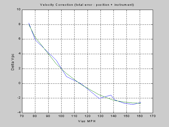
Using MATLAB to determine the coefficients of the polynomial fit, the equation for DV_pc(V_ias) is:

This equation is used to analytically determine DV_pc for all values of V_i throughout the clean configuration envelope.

For use in the cockpit a more useful tool is a plot of V_cas vs. V_ias as shown below in figure 2.

Figure 2 Vcas vs. Vias (mph)

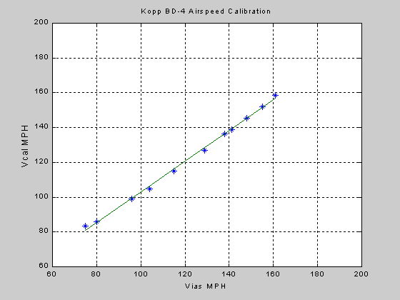
To obtain an analytic solution for V_cas at any V_ias a first order polynomial fit was used to generate the following equation:

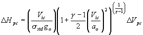
With this equation for DV_pc it is possible to determine DH_pc and DP_s from the following relationships derived in the NPS, AA4323 Flight Test Engineering Class notes:

, where DV_ic and DV_pc must be in ft/sec.

and

Close examination of the above two equations reveals DP_s to be insensitive to altitude and atmospheric conditions while DH_pc is affected by changes in altitude, as would be expected in an altimeter! Therefore, DH_pc must be determined for each altitude at which a flight test was conducted.

By substituting the 5^th order polynomial fit for DV_pc into the above two equations and iterating throughout the full range of airspeeds (V_i), the following plots and equations result:

Figure 3 Ps

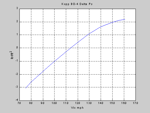
Where DP_s can be represented by:

using a 3^rd order polynomial fit of the plot in figure 3 above.

Iterating altitude from sea level to 10,000 pressure altitude results in DH_pc curves as shown below in figure 4.

Figure 4 Hpc Plot

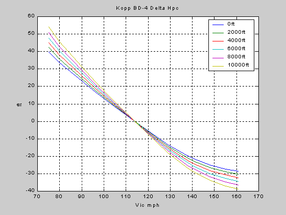
Where the DH_pc is also represented also by a 3^rd order polynomial fit equal to:

@ 1000 ft H_i

Otherwise for the general solution :

DH_pc(σ_std,V_ic)=

where

and

In truth the values DV_pc, DH_pc and DP_s for this airplane also include the instrumentation errors as data is not available for the errors of the instruments themselves. The important point however, is to determine the total system error and apply a correction to any further data collected.

Part II – Drag Polar / Power Required

In this section the findings from flight testing to determine the drag polar and power required for the Kopp BD-4 will be reported. Determination of an accurate drag polar enables the calculation of many vital performance metrics such as (L/D)_max, C_do, and the Oswald Span Efficiency Factor, e. Determination of power required curves provides both a graphical and analytic method for determination of other important parameters such as maximum range and endurance airspeed and minimum power required.

An aircraft drag polar is simply a plot of lift vs. drag or C_l vs. C_d for a particular configuration and is a measure of the aerodynamic efficiency of the complete aircraft independent of the installed propulsion source (to the extent the propulsion configuration contributes to added aircraft drag). Lift is the easiest quantity to determine since in level flight the total lift equals the gross weight of the aircraft at that instant in time. Drag however is quite difficult to measure with any accuracy in-flight without additional equipment. Fortunately, using proprietary software on loan from Hartzell Propeller Inc. 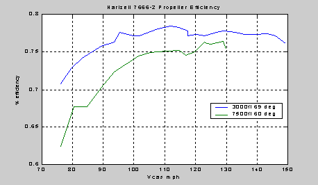determination of the 7666-2 blade efficiency and thrust generated was greatly simplified. To use this software the relationship of V_tas for given engine power settings, which is a combination of manifold pressure and propeller rpm, must be determined. Altitude and temperature are important inputs as well aircraft weight at the time of testing. This requires an accurate fuel-burn chart for calculation of weight as a function of time for each data point. The Lycoming O-360 operator’s manual includes both engine power and fuel-burn charts for use in computing the necessary information. Copies of these charts can be found in the appendix. Determination of power required as a function of airspeed is obtained using the data collected for the drag polar.

Flight Test Procedure

There are two basic methods for drag-polar data collection, the constant-airspeed and constant-altitude method. In the constant airspeed method the pilot flies a designated airspeed while power is adjusted as required to maintain altitude at that airspeed. Power, H_i, T_i and V_i, are recorded after all parameters have stabilized. This process is repeated over the full range of airspeeds in the designated configuration. Conversely the constant-altitude method requires the pilot to establish an altitude, set power to a desired level and adjust pitch attitude to maintain altitude. Once stabilized, the information is recorded and the next power setting adjusted. This process is repeated throughout a range of power settings. The constant-altitude method is beneficial at higher airspeeds because a power schedule can be developed and tabulated during pre-flight planning for organized data collection during flight. Additionally it is much easier to set a specified power setting and record the resulting airspeed than it is to fly an exact airspeed and determine the power setting. This is largely due to the size and scaling of the manifold pressure and rpm instrument face used for power determination. Because priory information of minimum power required for this particular airframe is not known, it is necessary to revert to the constant-airspeed method at lower airspeeds. To help ensure accurate data two runs are conducted for each airspeed / power combination. The data is averaged over both runs to arrive at one set of data for each altitude and weight of interest.

Drag Polar / Power Required Flight Test

This test was conducted in the Kopp BD-4 on 27 July, 2000 departing from Monterey Peninsula Airport (MRY) at 10:11 am. Conditions at take-off were:

Wind: 290/8

Alt: 30.04

Sky Clear

Rwy: 28R

It was determined during pre-flight planning that two separate runs would be made at different gross weights and altitudes. Crew and altitude assignments were as follows:

Table 3 Crew and altitude assignments

Crew	Altitude	Gross Weight (approx)
LT Ken Kopp / Maj. Jim Hawkins	3000 ft	1950 lbs
LT Ken Kopp / LT Anthony Fortesque	7500 ft	2150 lbs

The test area was restricted to the Salinas Valley from Salinas to 15 miles South East of King City. Crew coordination and a thorough test procedures briefing preceded each flight. Data collection sheets were developed, printed and discussed in detail prior to flight as well. Specific responsibilities were delegated as follows:

Table 4 Flight Responsibilities

Responsibility	Pilot at the Controls	Pilot Not at the Controls
Flight Safety	Primary	Secondary
Airwork	Primary
Test Procedure		Primary
Data Recording		Primary
Communications	Primary	Secondary
Navigation	Secondary	Primary
Visual Lookout	Secondary	Primary
Emergencies	Primary	Secondary

ATC flight following was utilized to the maximum extent possible to aid in collision

avoidance. King City and Salinas Muni were designated primary diverts in the event an emergency due to mechanical failure or weather occurred.

Each pilot was responsible for one run. At the completion of a run a control swap was accomplished and the second run completed. The results of the test conducted at 3000 feet pressure altitude are listed in table 5 below. 7000 feet data is included in the appendix.

Table 5. 3000 ft Data

Flight Test Data Sheet					Power Required					N375JK Kopp BD-4
st fuel	G W	Wind	Alt	Temp	Srt T	T/O T	C pwr	lvl T	trans pwr	C BR	GW	A br	Delt Time	final gw	Ave GW	Ts
33	1991.4	290/8	30.04	16	10:00	10:11	160	10:16	164	13	1984	7.8	63	1928.34	1956	50
Run #1	Ken				Test Data					Run #2	Jim			Test Data
MP	RPM	IAS	PA	OAT	Time	Ind HP	BR	GW	MP	RPM	IAS	PA	OAT	TIme	Ind HP	GW
26.5	2700	154	2995	69	2.0	163	13	1981	26.5	2700	154	3000	69	1.0	163	1927.0
26	2600	150	2995	68	2.0	159	13	1978	26	2600	150	3000	69	1.0	159	1928.4
25.5	2550	148	3000	68	1.0	152	11.5	1977	25.5	2550	146	3000	69	2.0	152	1929.9
25	2500	143	2995	68	1.0	146	11.5	1976	25	2500	142	3010	69	1.0	146	1932.5
24.5	2450	137	3000	66	2.0	140	11.5	1973	24.5	2450	140	3020	69	1.0	140	1933.8
24	2400	135	2998	67	2.0	132	8.8	1971	24	2400	135	3020	69	1.0	132	1935.1
23.5	2350	131	3000	68	1.0	124	8.8	1970	23.5	2350	131	3020	69	1.0	124	1936.1
23	2300	129	3000	68	1.0	120	8.8	1969	23	2300	129	3000	69	1.0	120	1937.1
22.5	2250	122	3000	68	1.0	114	7.5	1968	22.5	2250	125	3000	69	1.0	114	1938.1
22	2200	119	3000	68	1.0	108	7.5	1967	22	2200	122	3020	69	1.0	108	1939.0
21.5	2200	115	3000	70	2.0	104	7.5	1966	21.5	2200	120	3000	69	1.0	104	1939.8
21	2200	116	3000	69	2.0	100	6.3	1964	21	2200	119	2990	69	1.0	100	1940.7
20.5	2200	113	3000	69	2.0	96	6.3	1963	20.5	2200	115	3000	69	1.0	96	1941.4
20	2200	112	2995	69	1.0	92	6.3	1962	20	2200	110	3000	69	1.0	92	1942.1
19.5	2200	109	2995	69	1.0	89	6.3	1961	19.5	2200	104	3010	69	1.0	89	1942.8
19	2200	104	3000	69	2.0	86	6.3	1960	19	2200	95	3050	69	1.0	86	1943.5
18.5	2200	100	2995	69	1.0	82	5.5	1959	18.5	2200	94	3000	69	1.0	82	1944.2
18	2200	94	3000	69	3.0	78	5.5	1957	18	2200	90	2970	69	2.0	78	1944.9
18	2200	90	2995	68	2.0	78	5.5	1956	17	2200	88	3000	69	1.0	72	1946.1
17.5	2200	85	3000	68	2.0	74	5.5	1955	19	2200	76	3050	69	1.0	86	1946.7
17	2200	78	3000	69	1.0	72	5.5	1954	18	2200	70	2925	69	2.0	78	1947.4
17.5	2200	74	3050	68	3.0	74	5.5	1952
18	2200	70	3000	70	6.0	78	5.5	1949

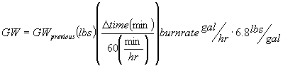
The top row of the table consists of starting weight, starting fuel, basic weather information, engine start time, take off time, climb power and level off time. These values are used to determine the fuel burned during t/o, climb and transit to the working area in order to calculate an accurate test start weight. The first six columns for each run are recorded data; manifold pressure, propeller rpm, indicated airspeed, pressure altitude, outside air temperature and the elapsed time between power changes. Engine power was determined through use of the manufacturers supplied engine power chart provided in the appendix. With engine HP recorded the fuel-burn chart, also included in the appendix, was entered and the corresponding value placed on the data sheet. A running reduction in aircraft gross weight was calculated according to the following relationship:

The excel spreadsheet shown in table 6 automatically links raw data from table 5 and calculates results for export to MATLAB for further analysis and plotting.

Table 6 Data Reduction for 3000 feet PA

Reduced Data for 3000 ft and 1950 lbs
1	2	3	4	5	6	7	8	9	10	11	12	13	14
MP	RPM	IAS	IAS	Ave IAS	AveGW	Vcas	Vtas	M	Ind HP	Corr HP	n	THP	Thrust
26.5	2700	154	154	154	1954.03	149.54	159.26	0.207	163	159.6	0.761	121.5	286
26	2600	150	150	150	1953.29	146.05	155.54	0.202	159	155.7	0.771	120.0	297
25.5	2550	148	146	147	1953.38	143.43	152.75	0.199	152	148.8	0.774	115.2	293
25	2500	143	142	142.5	1954.03	139.50	148.57	0.193	146	143.0	0.773	110.5	295
24.5	2450	137	140	138.5	1953.38	136.00	144.85	0.188	140	137.1	0.773	106.0	295
24	2400	135	135	135	1953.03	132.95	141.59	0.184	132	129.2	0.776	100.3	286
23.5	2350	131	131	131	1953.03	129.45	137.87	0.179	124	121.4	0.778	94.5	277
23	2300	129	129	129	1953.03	127.71	136.01	0.177	120	117.5	0.777	91.3	269
22.5	2250	122	125	123.5	1953.10	122.90	130.89	0.170	114	111.6	0.772	86.2	262
22	2200	119	122	120.5	1953.10	120.28	128.10	0.167	108	105.7	0.773	81.7	252
21.5	2200	115	120	117.5	1952.68	117.66	125.31	0.163	104	101.8	0.771	78.5	253
21	2200	116	119	117.5	1952.39	117.66	125.31	0.163	100	97.9	0.778	76.2	242
20.5	2200	113	115	114	1952.03	114.61	122.06	0.159	96	94.0	0.783	73.6	230
20	2200	112	110	111	1952.03	111.99	119.27	0.155	92	90.1	0.784	70.6	223
19.5	2200	109	104	106.5	1952.03	108.06	115.08	0.150	89	87.1	0.781	68.1	222
19	2200	104	95	99.5	1951.68	101.94	108.57	0.141	86	84.2	0.772	65.0	225
18.5	2200	100	94	97	1951.72	99.76	106.25	0.138	82	80.3	0.771	61.9	219
18	2200	94	90	92	1951.10	95.39	101.60	0.132	78	76.4	0.776	59.3	217
18	2200	90	90	90	1951.10	93.65	99.74	0.130	78	76.4	0.763	58.3	219
17.5	2200	85		85	1950.79	89.28	95.09	0.124	74	72.4	0.758	54.9	216
17	2200	78		78	1950.79	83.17	88.58	0.115	72	70.5	0.742	52.3	223
17.5	2200	74		74	1952.35	79.67	84.86	0.110	74	72.4	0.728	52.7	235
18	2200	70	70	70	1948.61	76.18	81.13	0.106	78	76.4	0.708	54.1	252
	Atmospheric Data		Temp		s sound	CAS Curve Fit
sigma	rstd	P3000	Ts	T	a	slope	intercept
0.88161	0.00237	1896.7	48.3	69	1127.33	0.87	15.05

Columns 1-4 are linked cells and are self explanatory as is column 5. Column 6 is the average gross weight of the aircraft at the time each data point was collected. V_cas in column 7 is derived from the curve fit data at the bottom of the table. The curve fit was obtained as discussed in the previous section. V_tas and Mach number are calculated for entry into the propeller thrust and efficiency software. Indicated HP was obtained from the engine chart . Because the Lycoming O-360-A1A is normally aspirated (fancy way of saying it uses a carburetor), the power generated is a function of the ratio of standard atmospheric temperature (at a specific pressure altitude) and the inlet temperature. For our purpose we will assume the OAT measurement of static ambient temperature is equal to the inlet temperature. In fact this may not be a reasonable assumption as inlet air passes many very hot engine components prior to fuel-air atomization. In effect this ratio is a measure of combustion efficiency and is calculated according to the following relationship:

, where T_s and T_i are given in °F.

If the altimeter had zero instrument error and it was known the static source was also error free, T_s would correspond to the standard temperature found in the atmosphere tables for the H_i (indicated pressure altitude) flown. However, as discussed in the previous section it is necessary to apply error corrections to H_i in order to obtain the true pressure altitude, H_c, flown at each test point. Once H_c is obtained the standard atmosphere tables can be used to retrieve the actual T_s and P_s through interpolation. With T_s determined for each data point a more accurate calculation of HP_corrected can be obtained. 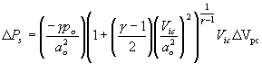P_s is used to calculate actual air density at H_c and T_i through use of the equation of state for a perfect gas as shown below.

. Density is a key factor in accurately determining the lift and drag coefficients C_L & C_D used extensively in performance analysis.

Through application of the equations derived in the previous sections and development of yet another spreadsheet the following corrections and values were obtained in table 7.

Table 7 Error Corrections for 3000 ft

3000ft	rho std	sigstd	gama	ao
	0.0022	0.918	1.4	1116.3
Ave Ias	Ave Alt	D Vpc	D Hpc	Hc	Ts	Ps	rho
154	2997.50	-2.44	-27.55	2969.95	47.23	1899.00	0.0020885
150	2997.50	-2.40	-26.34	2971.16	47.22	1898.92	0.0020884
147	3000.00	-2.34	-25.18	2974.82	47.21	1898.66	0.0020881
142.5	3002.50	-2.20	-23.00	2979.50	47.19	1898.34	0.0020878
138.5	3010.00	-2.03	-20.60	2989.40	47.16	1897.64	0.002087
135	3009.00	-1.84	-18.18	2990.82	47.15	1897.54	0.0020869
131	3010.00	-1.57	-15.06	2994.94	47.14	1897.25	0.0020866
129	3000.00	-1.42	-13.39	2986.61	47.17	1897.84	0.0020872
123.5	3000.00	-0.94	-8.48	2991.52	47.15	1897.49	0.0020869
120.5	3010.00	-0.64	-5.65	3004.35	47.10	1896.60	0.0020859
117.5	3000.00	-0.32	-2.74	2997.26	47.13	1897.09	0.0020864
117.5	2995.00	-0.32	-2.74	2992.26	47.15	1897.44	0.0020868
114	3000.00	0.08	0.70	3000.70	47.12	1896.85	0.0020862
111	2997.50	0.45	3.69	3001.19	47.12	1896.82	0.0020861
106.5	3002.50	1.05	8.21	3010.71	47.08	1896.15	0.0020854
99.5	3025.00	2.11	15.30	3040.30	46.98	1894.08	0.0020831
97	2997.50	2.52	17.88	3015.38	47.07	1895.82	0.002085
92	2985.00	3.45	23.14	3008.14	47.09	1896.33	0.0020856
90	2997.50	3.85	25.31	3022.81	47.04	1895.30	0.0020845
85	3025.00	4.99	30.98	3055.98	46.92	1892.98	0.0020819
78	2962.50	6.99	39.76	3002.26	47.11	1896.74	0.002086
74	3050.00	8.41	45.38	3095.38	46.78	1890.22	0.0020789
70	3000.00	10.09	51.54	3051.54	46.94	1893.29	0.0020822
					Interpolation Values for 3000 ft
					A	Ts	Ps
					2500	509.77	1931.9
					3500	506.21	1861.9

Referring back to table 6, HP_corrected can now more accurately be solved with the calculated values of T_s listed above.

With Mach number, altitude, rpm, HP_corrected and T_i, Hartzell’s propeller software is used to generate the efficiency and thrust generated by the propeller. The software contains proprietary performance maps of the 7666-2 blade generated through many hours of ground and flight testing and assumes a .4 blockage factor in thrust calculations. Because Lycoming engines are of the direct drive category, meaning engine crankshaft and propeller are connected directly and turns at the same rate, HP_corrected is equivalent to the more commonly used term Shaft Horsepower or SHP. Engines equipped with reduction drives must account for less than 100% power delivery to the propeller in calculations of SHP.

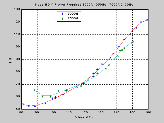
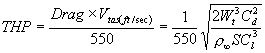
With SHP determined and software generated propeller efficiency in hand, it is now possible to determine the actual power delivered to the airframe by the engine / propeller combination. This power is referred to as Thrust Horsepower or THP and is determined by the simple relationship shown below:

, where η is propeller efficiency and is precisely how values in column 13 of table 6 were determined. Column 14 lists the thrust calculated by the Hartzell program as a function of V_tas. The software generated thrust is determined based on a standard fuselage blockage factor of approximately .4. This results in thrust values while representative of the actual thrust developed by the propeller they are higher than the thrust required by the airframe to maintain level flight. This is an important distinction if the power required data generated is to remain independent of the propulsive system installed. The thrust (drag) required by the airframe is calculated then from the equation below.

A plot of the propeller generated thrust and airframe required thrust clearly illustrates the effect of the inclusion of blockage factor during thrust calculation.

Figure 5 Propeller Thrust vs. Airframe Thrust Required

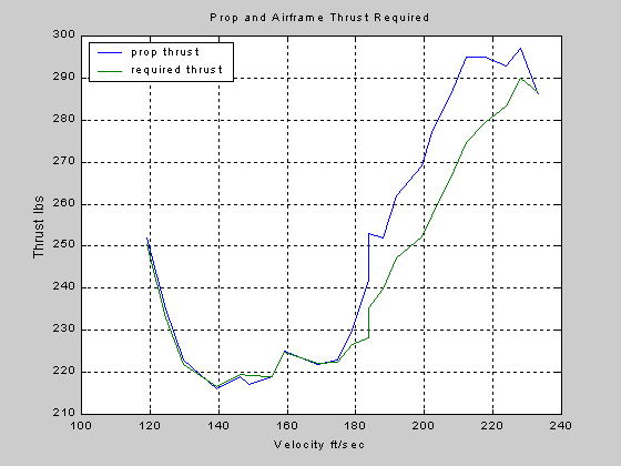
As may be expected as velocity increases the effect of fuselage blockage becomes greater as highlighted in the plot. All remaining calculations will be based on the airframe required thrust calculated according to the equation described on the previous page.

Data Analysis

Drag Polar

As discussed previously the drag polar is a measure of an airframes aerodynamic efficiency independent of the installed propulsion system and is generated by plotting Lift vs. Drag. Because total lift and drag are cumbersome terms it is common to plot the drag polar as a function of the non-dimensional lift and drag coefficients, C_l and C_d according to the following relationships:

, where V_{∞ is} V_tas is ft/sec and S is the total aircraft wing area .

and

, recalling basic Newtonian physics; in level unaccelerated flight the airplane is in equilibrium, therefore:

and shown pictorially below.

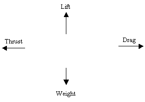
Thus, lift = weight and drag = thrust. Substitution of these equalities leads to:

and .

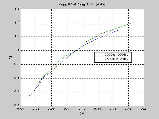
The drag polar can now be plotted from our tabulated data obtained during flight test and as shown in figure 6 below.

Figure 6 Drag Polar

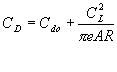
Another method for determining the drag coefficient is provided by finite wing theory, which predicts C_d to be equal to the sum of parasite and induced drag given by the following equation.

induced drag

parasite drag

, where C_do is the zero lift drag coefficient, e is the Oswald Span Efficiency Factor and accounts for non-elliptical shaped wing planforms and the contribution to parasite drag due to lift[3]. AR is the wing aspect ratio calculated as:

, where b is wing span and S is total wing area.

Determination of an accurate C_do is an important step in the design process of all aircraft. Parasite drag is the major source of drag at high speeds and therefore must be determined early in the design phase for accurate engine sizing, weight determination and performance calculations. For an airplane still on the design table, detailed methods have been developed by aerospace manufactures to estimate C_do through elaborate accounting of parasite drag of all wetted components. Thankfully the benefit of a fully functional airplane allows us to solve for C_do and e directly from flight test data. 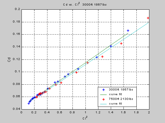This also provides a means to double check the theory as an academic exercise. Recalling the finite wing theory equation for C_d as

, notice that C_D is linear in C_L² !

C_d and C_l have been determined previously from flight test data and plotted in figure 5 as a drag polar. All that remains is to plot C_D as a function of C_L² and determine the slope and intercept for e and C_do respectively. C_D vs C_L² is shown in figure 7.

Figure 7 Cd vs. Cl^2

Data for both the 3000 ft 1950 lb and 7500ft 2130 lbs case converge nicely showing that values of e and C_do are relatively insensitive to atmospheric and weight changes . Using MATLAB to determine the slope and intercept of these two curves results in:

Altitude	Oswald Span Efficiency	Cdo
3000 ft	.7039	0.0440
7500 ft	.7289	0.0433

Table 8 Cdo and e

with e and C_do for each altitude C_d is recalculated according to the finite wing equation and a new drag polar plotted based on the theory as shown below in figure 8.

Figure 8 Calculated Drag Polar

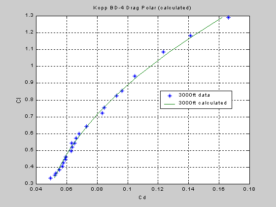
Clearly the theory does an excellent job of determining the drag coefficient from calculated values of C_do and e.

Recalling the free-body diagram depicted on page 26, from the equilibrium sum of forces during level unaccelerated flight where lift=weight and drag=thrust we can derive an important relationship as follows:

and where , where

Therefore:

, Thus

, from this equation it is apparent that minimum thrust required to maintain level unaccelerated flight occurs when the ratio C_l/C_d is a maximum!

Because values for C_l and C_d have been calculated from the data it is a simple matter of choosing the largest value of the resulting ratio. Using MATLAB to carry out this calculation results in values of:

Table 9. Max Lift / Drag

Altitude / Weight	Max Cl/Cd	Min Thrust Required
3000 ft / 1950 lbs	8.955	217.87 lbs
7500 ft / 2130 lbs	9.1957	229.63 lbs

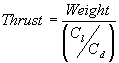
Referring back to table 6 for the reduced data at 3000 ft shows the recorded minimum thrust (highlighted in red) to be 222 lbs, thus providing excellent correlation with the theoretical value predicted in table 9 above. Another useful means for determination of (L/D)_max is simply graphing the ratio and noting the value at which point a maximum occurs as depicted in figure 9 on the next page.

For a given airspeed C_l must increase with gross weight to maintain lift necessary for level flight. Concurrently as C_l increases C_d increases as a function of C_l², the net result of which is that (L/D)_max remains constant but the airspeed corresponding to (L/D)_max increases for an increasing gross weight. The .24 difference in (L/D)_max calculated in table 9 may be attributed to instrument and other errors introduced during data collection.

Figure 9 Cl / Cd

Additionally, the point at which a line drawn from the origin and tangent to the drag polar curve intersects is also the point of (L/D)_max.

With the drag polar plot accurately determined many performance factors can now be analyzed as will be discussed in subsequent sections.

Power-required

For propeller driven aircraft determination of power-required for level unaccelerated flight constitutes a critical step toward performance measurement, prediction and optimization. The values obtained in this analysis directly impact the operational procedures used by the pilot to fly a particular mission profile. For example, power-required data provides the means to determine maximum range airspeed, a critical performance factor for flights over open water where distances between airfields may be great. Minimum power-required leads to maximum endurance airspeed. Critical for missions requiring long loiter times, such as patrol and search operations. The combination of power-required and power available data leads to performance calculations for climb rate, maximum airspeed, altitude performance effects and others. From a pilots perspective power-required determination is the single most important flight test data for real-time operational use.

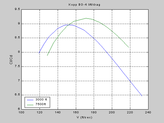
In actuality, power-required data was compiled when the thrust horsepower THP was determined while deriving the drag polar. All that remains is to plot THP vs. V_tas for a graphical representation of this airplanes power-required as shown in figure 10 on the next page.

Figure 10 THP vs Vtas (mph)

The high altitude, high weight configuration results in a shift of the power-required curve up and to the right. As altitude increases the minimum power-required increases while (L/D)_max remains constant. The effect of increased weight is higher minimum power-required and at higher velocity. Minimum power-required to maintain level unaccelerated flight is simply the lowest point of each curve. The values determined from curve fit are:

Table 10 Minimum Power-required

Altitude	Minimum Thrust Horsepower-required
3500 ft 1950 lbs	52.385 HP
7500 ft 2130 lbs	60.590 HP

Although these plots are useful in determining the performance parameters mentioned at the beginning of this section it would be necessary to derive a curve for each altitude and weight of interest due to their dependence on these parameters as shown above. To alleviate this tedious dilemma, development of normalized power-required vs. normalized airspeed reduces the data such that the resultant curve is independent of weight and altitude. In effect, one curve fits all.[4] Once this curve is generated a simple algorithm is used to extrapolate the data and a table of performance parameters for specific weights and altitudes is generated. The normalized parameters P_iw & V_iw are power and calibrated (M=.3 and below) airspeed corrected to standard weight sea level conditions. Where standard weight, W_s is defined as the maximum gross take-off weight for propeller driven aircraft.[5] For the Kopp BD-4 W_s = 2,200 lbs. Conversion of P_r & V_tas to their normalized values requires the following equations:

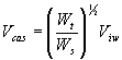
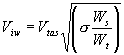, where W_t is the test weight.

for P_iw recall

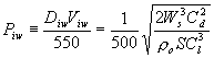and therefore

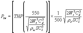
simplifying the above equation results in: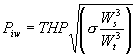

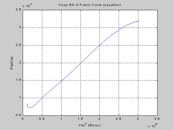
The normalized power required curve can now be plotted and performance parameters determined directly from the plot as shown below on figure 11.

Figure 11 Normalized Power Required

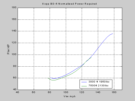
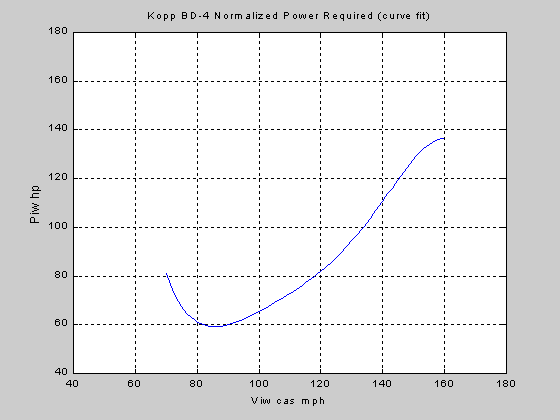
Ideally each curve for different weights and altitudes should converge into a single normalized curve. Unaccounted errors in propeller efficiency, oat instruments, MP and rpm can account for the slightly inconsistent results. Based on purely qualitative analysis of the conduct of the flight test it was determined the data recorded during the 3000 ft 1950 lbs gross weight run is the more accurate and will therefore be used to derive a 5^th order polynomial fit to provide a working equation by which to calculate the remaining parameters. MATLAB was used to generate the curve fit as follows:

Iterating the above equation for a range of V_iw from 70 -160 mph results in the curve fit plot of normalized power required shown in figure 12 below.

Figure 12 Normalized Power Required (curve fit)

max endurance airspeed

The next step is to determine the maximum range and endurance normalized airspeeds. This can be done graphically by drawing a line from the origin to a point of tangency along the Piw curve, the intersection of which corresponds to the maximum range normalized airspeed. Maximum endurance airspeed occurs at the minimum power required for level unaccelerated flight and is easily determined graphically by selecting the lowest point on the curve or analytically by differentiating the curve fit normalized power curve, equating to zero and solving for velocity. For propeller driven aircraft maximum range and endurance airspeed occur at (C_l/C_d)_max and (C_l^3/2/C_d)max. For use of the normalized curve normalized values of C_l and C_d must be calculated. C_l is calculated using W_s and sea level density, ρ_∞, throughout the speed range of interest. C_d is calculated as done previously using the finite wing theory equation for total airplane drag: 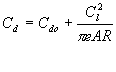. To ensure this method is valid values of C_do and e can be determined by plotting the linear equation:

P_iwV_iw = A₁V_iw⁴ + B₁ , called the Power Curve, and compared the values determined from the drag polar. By calculating values for the slope and intercept as A₁ and B₁ respectively and solving for C_do and e according to the following relationships:

and total Cd can be determined.

Again ratios Cl/Cd and Cl^3/2/Cd can be plotted. The maximum of each is located and the value of C_l corresponding to each is used to solve for the normalized airspeeds in question. The desired results are calibrated maximum range and endurance airspeed. With this, the total position error term DV_pc can be subtracted to retrieve indicated airspeed as seen by the pilot in flight. To illustrate this method maximum range airspeed will be determined in this fashion.

The power curve is plotted below:

Figure 13 Power Curve

from the plot and equations listed on the previous page C_do and e are calculated and compared to the values determined from the drag polar in table 11 below :

Parameters	Drag Polar	Power Curve
Cdo	0.0440	0.0425
e	0.7031	0.6507

Table 11Cdo and e comparisons

These values show good correlation to those calculated via the drag polar.

The normalized drag polar plotted below is used to determine normalized (Cl/Cd)_max

and corresponding value of C_l .

Figure 14 Normalized Drag Polar

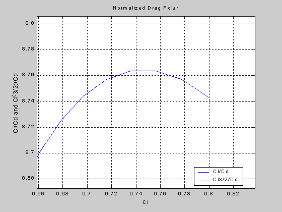
C_l at (Cl/Cd)_max is .744. Solving for V_iw with this value by

which corresponds nicely to the tangent drawn to the normalized power required curve in figure 11. Because V_cas for max range is a function of (L/D)_max and remains constant with changes in altitude, variations in V_cas for max range and endurance are dependent on weight changes only. Therefore, maximum range V_cas for any weight is given by:

therefore the maximum range airspeed at the first test condition weight of 1950 lbs = 100.23 mph calibrated.

Maximum normalized endurance airspeed is determined by locating the airspeed corresponding to the minimum power required. Referring back to figure 11 for the normalized power required curve reveals 85.5 mph calibrated normalized airspeed gives maximum endurance performance in the Kopp BD-4. Applying the equation above:

V_{cas endurance}= 80.49 mph @ 1950 lbs.

The real utility in this approach is the ease in which a performance table can be constructed within a spreadsheet program as displayed below.

Table 12 Performance Table

			Airspeed	Correction
Vias	65.0	70.0	75.0	80.0	85.0	90.0	95.0
Vcas	71.6	76.0	80.3	84.7	89.0	93.4	97.7
Vias	100.0	105.0	110.0	115.0	120.0	125.0	130.0
Vcas	102.1	106.4	110.8	115.1	119.5	123.8	128.2
Vias	135.0	140.0	145.0	150.0	155.0	160.0	165.0
Vcas	132.5	136.9	141.2	145.6	149.9	154.3	158.6
Vias	170.0	175.0	180.0
Vcas	163.0	167.3	171.7
			Vcas
G Weight	1600	1700	1800	1900	2000	2100	2200
Range	90.8	93.6	96.3	98.9	101.5	104.0	106.5
Endurance	72.9	75.2	77.3	79.5	81.5	83.5	85.5
			Vias
G. Weight	1600	1700	1800	1900	2000	2100	2200
Range	87.1	90.3	93.4	96.4	99.4	102.3	105.1
Endurance	66.5	69.1	71.6	74.0	76.4	78.7	81.0

The normalized power transformation has utility in an ability to predict the minimum power required for various altitudes and gross weights and can be used to determine the maximum sustainable altitude as illustrated below.

To determine if the Kopp BD-4 can maintain level flight at an altitude of 15,000 feet at max gross weight (2200lbs) use the following relationships:

σ @ 15K feet = .6313 therefore;

Consultation of the power chart and propeller efficiency software reveals a THP_available equal to only 71.09 hp. Therefore, at max gross weight the Kopp BD-4 will not be capable of maintaining an altitude of 15,000 feet. A gross weight of 2,000 lbs requires 70.99 hp at 15,000 ft, which should be attainable for standard day conditions. It will be interesting to investigate this prediction during flight test!

Summary and Conclusions

In this test key instrument calibration correction factors were developed and applied, thereby providing means for more accurate data analysis in subsequent testing. Applying FAA standards for certified aircraft for a maximum DV_pc 0f +- 6 mph shows the Kopp BD-4 to be skirting the limit throughout most of its airspeed range. Further testing of the instrumentation and aircraft are warranted in this matter. Also, an attempt to obtain manufacturer calibration errors may improve the results as well. Development of the drag polar, power required curves and Cl/Cd provided valuable information immediately usable by the pilot (that’s me!). A summary table below highlights many of the details resulting from this effort. Further testing will provide even greater insight into the performance and characteristics of this versatile little airplane.

Table 13 Summary

Altitude / Weight	Max Cl/Cd	Min Thrust Required
3000 ft / 1950 lbs	8.8235	217.87 lbs
7500 ft / 2130 lbs	9.0329	229.63 lbs
Parameters	Drag Polar	Power Curve
Cdo	0.0440	0.0425
e	0.7031	0.6507
Altitude	Minimum Thrust Horsepower Required
3500 ft 1950 lbs	52.33 HP
7500 ft 2130 lbs	60.59 HP
Standardized	59.16 HP
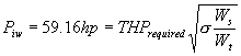
Kopp BD-4 Summary Table Test conducted 27 July, 2000 Data to be added upon further testing

Finally, recalling the specific objectives listed in the introduction:

• Determine instrument accuracies (DV_pc & DH_pc)
• Determine the Drag Polar (C_L vs. C_D)
• Develop Power Required Curves
• Estimate (L/D)_max
• Determine minimum power required, maximum range and endurance airspeeds.

Clearly all objectives were met during this flight test. Flight Test II will investigate power-available and excess power. The combination of both sets of data will enable a vast array of performance calculations to be made.

Appendix A

Table 14 7500 ft Data and Reduction

Reduced Data for 7500 ft and 2130 lbs
		run 1	run 2
MP	RPM	IAS	IAS	Ave IAS	Ave GW	Vcas	Vtas	M	HP	Corr HP	n	THP	Thrust
22.7	2700	129	134	131.5	2128.38	129.78	150.39	0.197	142	138.0	0.754	104.1	259
22.7	2600	130	131	130.5	2125.77	128.91	149.37	0.196	139	135.1	0.764	103.2	267
22.7	2500	126	126	126	2123.28	124.98	144.82	0.190	134	130.2	0.76	99.0	272
22.7	2450	124	125	124.5	2122.28	123.67	143.30	0.188	132	128.3	0.761	97.6	265
22.7	2400	123	124	123.5	2121.28	122.80	142.29	0.187	131	127.3	0.763	97.1	259
22.7	2300	121	123	122	2120.29	121.49	140.77	0.185	126	122.4	0.758	92.8	247
22.5	2250	120	120	120	2117.79	119.74	138.75	0.182	124	120.5	0.75	90.4	245
22	2200	117	116	116.5	2116.52	116.68	135.21	0.177	118	114.7	0.746	85.5	239
21.5	2200	115	114	114.5	2115.67	114.94	133.18	0.175	113	109.8	0.752	82.6	232
21	2200	109	110	109.5	2114.39	110.57	128.12	0.168	108	104.9	0.751	78.8	230
20	2200	103	104	103.5	2113.12	105.33	122.05	0.160	102	99.1	0.749	74.2	229
19	2200	99		99	2111.69	101.40	117.50	0.154	95	92.3	0.745	68.8	229
18.5	2200	90		90	2110.98	93.54	108.39	0.142	92	89.4	0.723	64.6	238
19.5	2200	85		85	2109.91	89.17	103.33	0.136	95	92.3	0.702	64.8	245
19	2200	80	76	78	2108.83	83.06	96.25	0.126	92	89.4	0.677	60.5	252
18.5	2200	75		75	2107.05	80.44	93.21	0.122	92	89.4	0.677	60.5	252
21	2200	70		70	2122.42	76.08	88.15	0.116	108	104.9	0.624	65.5	279
	Atmospheric Data		Temp		Sonic Speed	CAS Curve Fit
sigma	rstd	p7500	Ts	T	a	slope	intercept
0.74477	0.00237	1602.3	32	60	1117.6976	0.8733	14.9441

Flight Test Data Sheet			7500ft		Power Required					N375JK Kopp BD-4
GW	fuel	Wind	Alt	T	Srt T	T/O T	C pwr	lvl T	trans pwr	C br	GW	A br	Delt Time	final gw	Ave GW	Ts
2168	56	290/8	30.04	17	12:30	12:39	160	12:53	164	13	2147	8	66	2089.0	2118	46
Run #1	Ken		Test Data							Run #2	Ant		Test Data
MP	RPM	IAS	PA	OAT	Time	HP	BR	GW	MP	RPM	IAS	PA	OAT	TIme	HP	GW
22.7	2700	129	7500	60	0.0	142	11.5	2147.4	22.7	2700	134	7500	60	10.0	142	2109.4
22.7	2600	130	7500	60	3.0	139	11.5	2143.5	22.7	2600	131	7500	60	1.0	139	2108.1
22.7	2500	126	7500	60	3.0	134	8.8	2140.5	22.7	2500	126	7500	60	2.0	134	2106.1
22.7	2450	124	7500	60	1.0	132	8.8	2139.5	22.7	2450	125	7500	60	1.0	132	2105.1
22.7	2400	123	7500	60	1.0	131	8.8	2138.5	22.7	2400	124	7520	60	1.0	131	2104.1
22.7	2300	121	7500	60	1.0	126	8.8	2137.5	22.7	2300	123	7500	60	1.0	126	2103.1
22.5	2250	120	7500	60	3.0	124	8.8	2134.5	22.5	2250	120	7500	60	2.0	124	2101.1
22	2200	117	7500	60	2.0	118	7.5	2132.8	22	2200	116	7500	60	1.0	118	2100.2
21.5	2200	115	7500	60	1.0	113	7.5	2131.9	21.5	2200	114	7500	60	1.0	113	2099.4
21	2200	109	7500	60	1.0	108	7.5	2131.1	21	2200	110	7520	60	2.0	108	2097.7
20	2200	103	7500	60	1.0	102	7.5	2130.2	20	2200	104	7500	60	2.0	102	2096.0
19	2200	99	7500	60	1.0	95	6.3	2129.5	19	2200	85	7520	60	3.0	95	2093.9
18.5	2200	90	7500	60	1.0	92	6.3	2128.8	18.5	2200	80	7540	60	1.0	92	2093.1
19.5	2200	85	7480	60	1.0	99	6.3	2128.1	19	2200	76	7500	60	2.0	95	2091.7
19	2200	80	7500	60	1.0	95	6.3	2127.4	19.5	2200	70	7400	60	2.0	99	2090.3
18.5	2200	75	7500	60	1.0	92	6.3	2126.7	20.5	2200	65	7500	60	4.0	105	2087.4
21	2200	70	7500	60	5.0	108	7.5	2122.4

Appendix B

Table 15 Instrument Corrections for 7500 ft

7500ft	rho std	sigstd	gama	ao
	0.0019	0.80042	1.4	1116.288
Ave IAS	Ave Alt	Delt Vpc	delt Hpc	Hc	Ts	Ps	rho	rhostd
131.50	7500.00	-1.61	-17.74	7482.26	31.14	1603.68	0.001794	0.001899
130.50	7500.00	-1.53	-16.80	7483.20	31.14	1603.62	0.001794	0.001898
126.00	7500.00	-1.17	-12.34	7487.66	31.12	1603.35	0.001794	0.001898
124.50	7500.00	-1.03	-10.78	7489.22	31.12	1603.26	0.001794	0.001898
123.50	7510.00	-0.94	-9.72	7500.28	31.08	1602.58	0.001793	0.001897
122.00	7500.00	-0.79	-8.11	7491.89	31.11	1603.09	0.001794	0.001898
120.00	7500.00	-0.59	-5.92	7494.08	31.10	1602.96	0.001793	0.001898
116.50	7500.00	-0.21	-2.02	7497.98	31.09	1602.72	0.001793	0.001898
114.50	7500.00	0.02	0.24	7500.24	31.08	1602.59	0.001793	0.001897
109.50	7510.00	0.65	5.95	7515.95	31.02	1601.63	0.001792	0.001897
103.50	7500.00	1.49	12.88	7512.88	31.03	1601.81	0.001792	0.001897
99.00	7510.00	2.19	18.13	7528.13	30.98	1600.88	0.001791	0.001896
90.00	7520.00	3.85	29.02	7549.02	30.91	1599.61	0.00179	0.001895
85.00	7490.00	4.99	35.52	7525.52	30.99	1601.04	0.001791	0.001896
78.00	7450.00	6.99	45.59	7495.59	31.10	1602.87	0.001793	0.001898
75.00	7500.00	8.03	50.37	7550.37	30.90	1599.53	0.00179	0.001895
70.00	7500.00	10.09	59.09	7559.09	30.87	1599.00	0.001789	0.001894
					Interpolation Values for 7000 ft
					A	Ts	Ps	rhostd
					7000	493.73	1633.1	0.00193
					8000	490.17	1572.1	0.00187

Figure 15 Prop efficiency

---

[1] AA4323 Class Notes

[2] AA4323 Flight Test Engineering Class Notes

[3] Anderson, “Introduction To Flight”, Ch.6

[4] AA4323 Flight Test Engineering Class Notes

[5] AA4323 Flight Test Engineering Class Notes